Cross-entropy

In information theory, the cross-entropy between two probability distributions ${\displaystyle p}$ and ${\displaystyle q}$, over the same underlying set of events, measures the average number of bits needed to identify an event drawn from the set when the coding scheme used for the set is optimized for an estimated probability distribution ${\displaystyle q}$, rather than the true distribution ${\displaystyle p}$.

Definition

The cross-entropy of the distribution ${\displaystyle q}$ relative to a distribution ${\displaystyle p}$ over a given set is defined as follows:

$${\displaystyle H(p,q)=-\operatorname {E} _{p}[\log q],}$$

where ${\displaystyle E_{p}[\cdot ]}$ is the expected value operator with respect to the distribution ${\displaystyle p}$.

The definition may be formulated using the Kullback–Leibler divergence ${\displaystyle D_{\mathrm {KL} }(p\parallel q)}$, divergence of ${\displaystyle p}$ from ${\displaystyle q}$ (also known as the relative entropy of ${\displaystyle p}$ with respect to ${\displaystyle q}$).

$${\displaystyle H(p,q)=H(p)+D_{\mathrm {KL} }(p\parallel q),}$$

where ${\displaystyle H(p)}$ is the entropy of ${\displaystyle p}$.

For discrete probability distributions ${\displaystyle p}$ and ${\displaystyle q}$ with the same support ${\displaystyle {\mathcal {X}}}$, this means

${\displaystyle H(p,q)=-\sum _{x\in {\mathcal {X}}}p(x)\,\log q(x).}$   (Eq.1)

The situation for continuous distributions is analogous. We have to assume that ${\displaystyle p}$ and ${\displaystyle q}$ are absolutely continuous with respect to some reference measure ${\displaystyle r}$ (usually ${\displaystyle r}$ is a Lebesgue measure on a Borel σ-algebra). Let ${\displaystyle P}$ and ${\displaystyle Q}$ be probability density functions of ${\displaystyle p}$ and ${\displaystyle q}$ with respect to ${\displaystyle r}$. Then

$${\displaystyle -\int _{\mathcal {X}}P(x)\,\log Q(x)\,\mathrm {d} x=\operatorname {E} _{p}[-\log Q],}$$

and therefore

${\displaystyle H(p,q)=-\int _{\mathcal {X}}P(x)\,\log Q(x)\,\mathrm {d} x.}$   (Eq.2)

NB: The notation ${\displaystyle H(p,q)}$ is also used for a different concept, the joint entropy of ${\displaystyle p}$ and ${\displaystyle q}$.

Motivation

In information theory, the Kraft–McMillan theorem establishes that any directly decodable coding scheme for coding a message to identify one value ${\displaystyle x_{i}}$ out of a set of possibilities ${\displaystyle \{x_{1},\ldots ,x_{n}\}}$ can be seen as representing an implicit probability distribution ${\displaystyle q(x_{i})=\left({\frac {1}{2}}\right)^{\ell _{i}}}$ over ${\displaystyle \{x_{1},\ldots ,x_{n}\}}$, where ${\displaystyle \ell _{i}}$ is the length of the code for ${\displaystyle x_{i}}$ in bits. Therefore, cross-entropy can be interpreted as the expected message-length per datum when a wrong distribution ${\displaystyle q}$ is assumed while the data actually follows a distribution ${\displaystyle p}$. That is why the expectation is taken over the true probability distribution ${\displaystyle p}$ and not ${\displaystyle q.}$ Indeed the expected message-length under the true distribution ${\displaystyle p}$ is

$${\displaystyle \operatorname {E} _{p}[\ell ]=-\operatorname {E} _{p}\left[{\frac {\ln {q(x)}}{\ln(2)}}\right]}$$$${\displaystyle =-\operatorname {E} _{p}\left[\log _{2}{q(x)}\right]=-\sum _{x_{i}}p(x_{i})\,\log _{2}q(x_{i})}$$$${\displaystyle =-\sum _{x}p(x)\,\log _{2}q(x)=H(p,q).}$$

Estimation

There are many situations where cross-entropy needs to be measured but the distribution of ${\displaystyle p}$ is unknown. An example is language modeling, where a model is created based on a training set ${\displaystyle T}$, and then its cross-entropy is measured on a test set to assess how accurate the model is in predicting the test data. In this example, ${\displaystyle p}$ is the true distribution of words in any corpus, and ${\displaystyle q}$ is the distribution of words as predicted by the model. Since the true distribution is unknown, cross-entropy cannot be directly calculated. In these cases, an estimate of cross-entropy is calculated using the following formula:

$${\displaystyle H(T,q)=-\sum _{i=1}^{N}{\frac {1}{N}}\log _{2}q(x_{i})}$$

where ${\displaystyle N}$ is the size of the test set, and ${\displaystyle q(x)}$ is the probability of event ${\displaystyle x}$ estimated from the training set. In other words, ${\displaystyle q(x_{i})}$ is the probability estimate of the model that the i-th word of the text is ${\displaystyle x_{i}}$. The sum is averaged over the ${\displaystyle N}$ words of the test. This is a Monte Carlo estimate of the true cross-entropy, where the test set is treated as samples from ${\displaystyle p(x)}$.^{[ citation needed ]}

Relation to maximum likelihood

The cross entropy arises in classification problems when introducing a logarithm in the guise of the log-likelihood function.

The section is concerned with the subject of estimation of the probability of different possible discrete outcomes. To this end, denote a parametrized family of distributions by ${\displaystyle q_{\theta }}$, with ${\displaystyle \theta }$ subject to the optimization effort. Consider a given finite sequence of ${\displaystyle N}$ values ${\displaystyle x_{i}}$ from a training set, obtained from conditionally independent sampling. The likelihood assigned to any considered parameter ${\displaystyle \theta }$ of the model is then given by the product over all probabilities ${\displaystyle q_{\theta }(X=x_{i})}$. Repeated occurrences are possible, leading to equal factors in the product. If the count of occurrences of the value equal to ${\displaystyle x_{i}}$ (for some index ${\displaystyle i}$) is denoted by ${\displaystyle \#x_{i}}$, then the frequency of that value equals ${\displaystyle \#x_{i}/N}$. Denote the latter by ${\displaystyle p(X=x_{i})}$, as it may be understood as empirical approximation to the probability distribution underlying the scenario. Further denote by ${\displaystyle PP:={\mathrm {e} }^{H(p,q_{\theta })}}$ the perplexity, which can be seen to equal ${\textstyle \prod _{x_{i}}q_{\theta }(X=x_{i})^{-p(X=x_{i})}}$ by the calculation rules for the logarithm, and where the product is over the values without double counting. So $${\displaystyle {\mathcal {L}}(\theta$$ ;{\mathbf {x} })=\prod _{i}q_{\theta }(X=x_{i})=\prod _{x_{i}}q_{\theta }(X=x_{i})^{\#x_{i}}=PP^{-N}={\mathrm {e} }^{-N\cdot H(p,q_{\theta })}} or $${\displaystyle \log {\mathcal {L}}(\theta$$ ;{\mathbf {x} })=-N\cdot H(p,q_{\theta }).} Since the logarithm is a monotonically increasing function, it does not affect extremization. So observe that the likelihood maximization amounts to minimization of the cross-entropy.

Cross-entropy minimization

Main article: Cross-entropy method

Cross-entropy minimization is frequently used in optimization and rare-event probability estimation. When comparing a distribution ${\displaystyle q}$ against a fixed reference distribution ${\displaystyle p}$, cross-entropy and KL divergence are identical up to an additive constant (since ${\displaystyle p}$ is fixed): According to the Gibbs' inequality, both take on their minimal values when ${\displaystyle p=q}$, which is ${\displaystyle 0}$ for KL divergence, and ${\displaystyle \mathrm {H} (p)}$ for cross-entropy. In the engineering literature, the principle of minimizing KL divergence (Kullback's "Principle of Minimum Discrimination Information") is often called the Principle of Minimum Cross-Entropy (MCE), or Minxent.

However, as discussed in the article Kullback–Leibler divergence , sometimes the distribution ${\displaystyle q}$ is the fixed prior reference distribution, and the distribution ${\displaystyle p}$ is optimized to be as close to ${\displaystyle q}$ as possible, subject to some constraint. In this case the two minimizations are not equivalent. This has led to some ambiguity in the literature, with some authors attempting to resolve the inconsistency by restating cross-entropy to be ${\displaystyle D_{\mathrm {KL} }(p\parallel q)}$, rather than ${\displaystyle H(p,q)}$. In fact, cross-entropy is another name for relative entropy; see Cover and Thomas ^[1] and Good. ^[2] On the other hand, ${\displaystyle H(p,q)}$ does not agree with the literature and can be misleading.

Cross-entropy loss function and logistic regression

Cross-entropy can be used to define a loss function in machine learning and optimization. Mao, Mohri, and Zhong (2023) give an extensive analysis of the properties of the family of cross-entropy loss functions in machine learning, including theoretical learning guarantees and extensions to adversarial learning. ^[3] The true probability ${\displaystyle p_{i}}$ is the true label, and the given distribution ${\displaystyle q_{i}}$ is the predicted value of the current model. This is also known as the log loss (or logarithmic loss ^[4] or logistic loss ); ^[5] the terms "log loss" and "cross-entropy loss" are used interchangeably. ^[6]

More specifically, consider a binary regression model which can be used to classify observations into two possible classes (often simply labelled ${\displaystyle 0}$ and ${\displaystyle 1}$). The output of the model for a given observation, given a vector of input features ${\displaystyle x}$, can be interpreted as a probability, which serves as the basis for classifying the observation. In logistic regression, the probability is modeled using the logistic function ${\displaystyle g(z)=1/(1+e^{-z})}$ where ${\displaystyle z}$ is some function of the input vector ${\displaystyle x}$, commonly just a linear function. The probability of the output ${\displaystyle y=1}$ is given by $${\displaystyle q_{y=1}={\hat {y}}\equiv g(\mathbf {w} \cdot \mathbf {x} )={\frac {1}{1+e^{-\mathbf {w} \cdot \mathbf {x} }}},}$$ where the vector of weights ${\displaystyle \mathbf {w} }$ is optimized through some appropriate algorithm such as gradient descent. Similarly, the complementary probability of finding the output ${\displaystyle y=0}$ is simply given by $${\displaystyle q_{y=0}=1-{\hat {y}}.}$$

Having set up our notation, ${\displaystyle p\in \{y,1-y\}}$ and ${\displaystyle q\in \{{\hat {y}},1-{\hat {y}}\}}$, we can use cross-entropy to get a measure of dissimilarity between ${\displaystyle p}$ and ${\displaystyle q}$: $${\displaystyle H(p,q)\ =\ -\sum _{i}p_{i}\log q_{i}\ =\ -y\log {\hat {y}}-(1-y)\log(1-{\hat {y}}).}$$

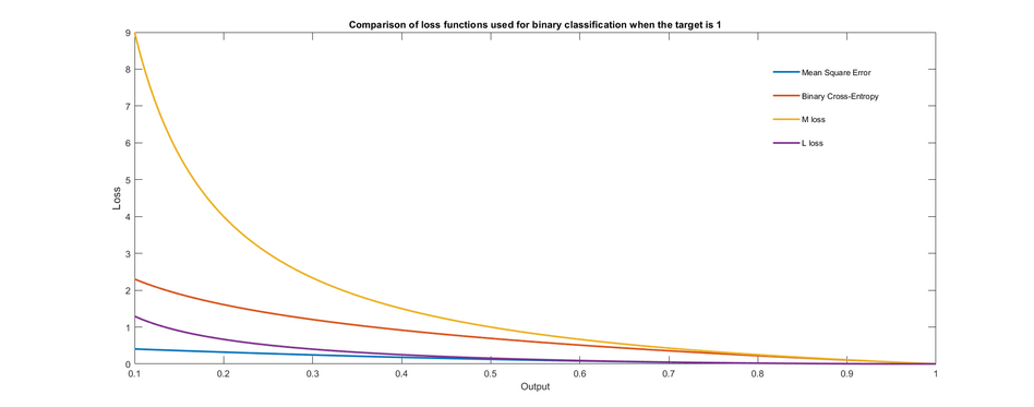
Plot shows different loss functions that can be used to train a binary classifier. Only the case where the target output is 1 is shown. It is observed that the loss is zero when the target is equal to the output and increases as the output becomes increasingly incorrect.

Logistic regression typically optimizes the log loss for all the observations on which it is trained, which is the same as optimizing the average cross-entropy in the sample. Other loss functions that penalize errors differently can be also used for training, resulting in models with different final test accuracy. ^[7] For example, suppose we have ${\displaystyle N}$ samples with each sample indexed by ${\displaystyle n=1,\dots ,N}$. The average of the loss function is then given by:

$${\displaystyle J(\mathbf {w} )\ =\ {\frac {1}{N}}\sum _{n=1}^{N}H(p_{n},q_{n})\ =\ -{\frac {1}{N}}\sum _{n=1}^{N}\ {\bigg [}y_{n}\log {\hat {y}}_{n}+(1-y_{n})\log(1-{\hat {y}}_{n}){\bigg ]}\,,}$$

where ${\displaystyle {\hat {y}}_{n}\equiv g(\mathbf {w} \cdot \mathbf {x} _{n})=1/(1+e^{-\mathbf {w} \cdot \mathbf {x} _{n}})}$, with ${\displaystyle g(z)}$ the logistic function as before.

The logistic loss is sometimes called cross-entropy loss. It is also known as log loss.^{[ duplication? ]} (In this case, the binary label is often denoted by {−1,+1}. ^[8] )

Remark: The gradient of the cross-entropy loss for logistic regression is the same as the gradient of the squared-error loss for linear regression. That is, define

$${\displaystyle X^{\mathsf {T}}={\begin{pmatrix}1&x_{11}&\dots &x_{1p}\\1&x_{21}&\cdots &x_{2p}\\\vdots &\vdots &&\vdots \\1&x_{n1}&\cdots &x_{np}\\\end{pmatrix}}\in \mathbb {R} ^{n\times (p+1)},}$$$${\displaystyle {\hat {y_{i}}}={\hat {f}}(x_{i1},\dots ,x_{ip})={\frac {1}{1+\exp(-\beta _{0}-\beta _{1}x_{i1}-\dots -\beta _{p}x_{ip})}},}$$$${\displaystyle L({\boldsymbol {\beta }})=-\sum _{i=1}^{N}\left[y_{i}\log {\hat {y}}_{i}+(1-y_{i})\log(1-{\hat {y}}_{i})\right].}$$

Then we have the result

$${\displaystyle {\frac {\partial }{\partial {\boldsymbol {\beta }}}}L({\boldsymbol {\beta }})=X^{T}({\hat {Y}}-Y).}$$

The proof is as follows. For any ${\displaystyle {\hat {y}}_{i}}$, we have

$${\displaystyle {\frac {\partial }{\partial \beta _{0}}}\ln {\frac {1}{1+e^{-\beta _{0}+k_{0}}}}={\frac {e^{-\beta _{0}+k_{0}}}{1+e^{-\beta _{0}+k_{0}}}},}$$$${\displaystyle {\frac {\partial }{\partial \beta _{0}}}\ln \left(1-{\frac {1}{1+e^{-\beta _{0}+k_{0}}}}\right)={\frac {-1}{1+e^{-\beta _{0}+k_{0}}}},}$$$${\displaystyle {\begin{aligned}{\frac {\partial }{\partial \beta _{0}}}L({\boldsymbol {\beta }})&=-\sum _{i=1}^{N}\left[{\frac {y_{i}\cdot e^{-\beta _{0}+k_{0}}}{1+e^{-\beta _{0}+k_{0}}}}-(1-y_{i}){\frac {1}{1+e^{-\beta _{0}+k_{0}}}}\right]\\&=-\sum _{i=1}^{N}\left[y_{i}-{\hat {y}}_{i}\right]=\sum _{i=1}^{N}({\hat {y}}_{i}-y_{i}),\end{aligned}}}$$$${\displaystyle {\frac {\partial }{\partial \beta _{1}}}\ln {\frac {1}{1+e^{-\beta _{1}x_{i1}+k_{1}}}}={\frac {x_{i1}e^{k_{1}}}{e^{\beta _{1}x_{i1}}+e^{k_{1}}}},}$$$${\displaystyle {\frac {\partial }{\partial \beta _{1}}}\ln \left[1-{\frac {1}{1+e^{-\beta _{1}x_{i1}+k_{1}}}}\right]={\frac {-x_{i1}e^{\beta _{1}x_{i1}}}{e^{\beta _{1}x_{i1}}+e^{k_{1}}}},}$$$${\displaystyle {\frac {\partial }{\partial \beta _{1}}}L({\boldsymbol {\beta }})=-\sum _{i=1}^{N}x_{i1}(y_{i}-{\hat {y}}_{i})=\sum _{i=1}^{N}x_{i1}({\hat {y}}_{i}-y_{i}).}$$

In a similar way, we eventually obtain the desired result.

Amended cross-entropy

It may be beneficial to train an ensemble of models that have diversity, such that when they are combined, their predictive accuracy is augmented. ^{[9] [10]} Assuming a simple ensemble of ${\displaystyle K}$ classifiers is assembled via averaging the outputs, then the amended cross-entropy is given by $${\displaystyle e^{k}=H(p,q^{k})-{\frac {\lambda }{K}}\sum _{j\neq k}H(q^{j},q^{k})}$$ where ${\displaystyle e^{k}}$ is the cost function of the ${\displaystyle k^{th}}$ classifier, ${\displaystyle q^{k}}$ is the output probability of the ${\displaystyle k^{th}}$ classifier, ${\displaystyle p}$ is the true probability to be estimated, and ${\displaystyle \lambda }$ is a parameter between 0 and 1 that defines the 'diversity' that we would like to establish among the ensemble. When ${\displaystyle \lambda =0}$ we want each classifier to do its best regardless of the ensemble and when ${\displaystyle \lambda =1}$ we would like the classifier to be as diverse as possible.

See also

• Cross-entropy method
• Logistic regression
• Conditional entropy
• Kullback–Leibler distance
• Maximum-likelihood estimation
• Mutual information
• Perplexity

References

1. Thomas M. Cover, Joy A. Thomas, Elements of Information Theory, 2nd Edition, Wiley, p. 80
2. I. J. Good, Maximum entropy for hypothesis formulation, especially for multidimensional contingency tables, Ann. of Math. Statistics, 1963
3. Anqi Mao, Mehryar Mohri, Yutao Zhong. Cross-entropy loss functions: Theoretical analysis and applications. ICML 2023. https://arxiv.org/pdf/2304.07288.pdf
4. The Mathematics of Information Coding, Extraction and Distribution, by George Cybenko, Dianne P. O'Leary, Jorma Rissanen, 1999, p. 82
5. Probability for Machine Learning: Discover How To Harness Uncertainty With Python, Jason Brownlee, 2019, p. 220: "Logistic loss refers to the loss function commonly used to optimize a logistic regression model. It may also be referred to as logarithmic loss (which is confusing) or simply log loss."
6. sklearn.metrics.log_loss
7. Noel, Mathew; Banerjee, Arindam; D, Geraldine Bessie Amali; Muthiah-Nakarajan, Venkataraman (March 17, 2023). "Alternate loss functions for classification and robust regression can improve the accuracy of artificial neural networks". arXiv: 2303.09935 [cs.NE].
8. Murphy, Kevin (2012). Machine Learning: A Probabilistic Perspective. MIT. ISBN   978-0262018029.
9. Shoham, Ron; Permuter, Haim H. (2019). "Amended Cross-Entropy Cost: An Approach for Encouraging Diversity in Classification Ensemble (Brief Announcement)". In Dolev, Shlomi; Hendler, Danny; Lodha, Sachin; Yung, Moti (eds.). Cyber Security Cryptography and Machine Learning – Third International Symposium, CSCML 2019, Beer-Sheva, Israel, June 27–28, 2019, Proceedings. Lecture Notes in Computer Science. Vol. 11527. Springer. pp. 202–207. doi:10.1007/978-3-030-20951-3_18. ISBN   978-3-030-20950-6.
10. Shoham, Ron; Permuter, Haim (2020). "Amended Cross Entropy Cost: Framework For Explicit Diversity Encouragement". arXiv: 2007.08140 [cs.LG].

Further reading

• de Boer, Kroese, D.P., Mannor, S. and Rubinstein, R.Y. (2005). A tutorial on the cross-entropy method. Annals of Operations Research 134 (1), 19–67.