Cyclostationary process

Last updated

A cyclostationary process is a signal having statistical properties that vary cyclically with time. [1] A cyclostationary process can be viewed as multiple interleaved stationary processes. For example, the maximum daily temperature in New York City can be modeled as a cyclostationary process: the maximum temperature on July 21 is statistically different from the temperature on December 20; however, it is a reasonable approximation that the temperature on December 20 of different years has identical statistics. Thus, we can view the random process composed of daily maximum temperatures as 365 interleaved stationary processes, each of which takes on a new value once per year.

Contents

Definition

There are two differing approaches to the treatment of cyclostationary processes. [2] The stochastic approach is to view measurements as an instance of an abstract stochastic process model. As an alternative, the more empirical approach is to view the measurements as a single time series of data--that which has actually been measured in practice and, for some parts of theory, conceptually extended from an observed finite time interval to an infinite interval. Both mathematical models lead to probabilistic theories: abstract stochastic probability for the stochastic process model and the more empirical Fraction Of Time (FOT) probability for the alternative model. The FOT probability of some event associated with the time series is defined to be the fraction of time that event occurs over the lifetime of the time series. In both approaches, the process or time series is said to be cyclostationary if and only if its associated probability distributions vary periodically with time. However, in the non-stochastic time-series approach, there is an alternative but equivalent definition: A time series that contains no finite-strength additive sine-wave components is said to exhibit cyclostationarity if and only if there exists some nonlinear time-invariant transformation of the time series that produces finite-strength (non-zero) additive sine-wave components.

Wide-sense cyclostationarity

An important special case of cyclostationary signals is one that exhibits cyclostationarity in second-order statistics (e.g., the autocorrelation function). These are called wide-sense cyclostationary signals, and are analogous to wide-sense stationary processes. The exact definition differs depending on whether the signal is treated as a stochastic process or as a deterministic time series.

Cyclostationary stochastic process

A stochastic process of mean and autocorrelation function:

where the star denotes complex conjugation, is said to be wide-sense cyclostationary with period if both and are cyclic in with period i.e.: [2]

The autocorrelation function is thus periodic in t and can be expanded in Fourier series:

where is called cyclic autocorrelation function and equal to:

The frequencies are called cycle frequencies.

Wide-sense stationary processes are a special case of cyclostationary processes with only .

Cyclostationary time series

A signal that is just a function of time and not a sample path of a stochastic process can exhibit cyclostationarity properties in the framework of the fraction-of-time point of view. This way, the cyclic autocorrelation function can be defined by: [2]

If the time-series is a sample path of a stochastic process it is . If the signal is further cycloergodic, [3] all sample paths exhibit the same cyclic time-averages with probability equal to 1 and thus with probability 1.

Frequency domain behavior

The Fourier transform of the cyclic autocorrelation function at cyclic frequency α is called cyclic spectrum or spectral correlation density function and is equal to:

The cyclic spectrum at zero cyclic frequency is also called average power spectral density. For a Gaussian cyclostationary process, its rate distortion function can be expressed in terms of its cyclic spectrum. [4]

The reason is called the spectral correlation density function is that it equals the limit, as filter bandwidth approaches zero, of the expected value of the product of the output of a one-sided bandpass filter with center frequency and the conjugate of the output of another one-sided bandpass filter with center frequency , with both filter outputs frequency shifted to a common center frequency, such as zero, as originally observed and proved in. [5]

For time series, the reason the cyclic spectral density function is called the spectral correlation density function is that it equals the limit, as filter bandwidth approaches zero, of the average over all time of the product of the output of a one-sided bandpass filter with center frequency and the conjugate of the output of another one-sided bandpass filter with center frequency , with both filter outputs frequency shifted to a common center frequency, such as zero, as originally observed and proved in. [6]

Example: linearly modulated digital signal

An example of cyclostationary signal is the linearly modulated digital signal  :

where are i.i.d. random variables. The waveform , with Fourier transform , is the supporting pulse of the modulation.

By assuming and , the auto-correlation function is:

The last summation is a periodic summation, hence a signal periodic in t. This way, is a cyclostationary signal with period and cyclic autocorrelation function:

with indicating convolution. The cyclic spectrum is:

Typical raised-cosine pulses adopted in digital communications have thus only non-zero cyclic frequencies.


This same result can be obtained for the non-stochastic time series model of linearly modulated digital signals in which expectation is replaced with infinite time average, but this requires a somewhat modified mathematical method as originally observed and proved in. [7]

Cyclostationary models

It is possible to generalise the class of autoregressive moving average models to incorporate cyclostationary behaviour. For example, Troutman [8] treated autoregressions in which the autoregression coefficients and residual variance are no longer constant but vary cyclically with time. His work follows a number of other studies of cyclostationary processes within the field of time series analysis. [9] [10]

Polycyclostationarity

In practice, signals exhibiting cyclicity with more than one incommensurate period arise and require a generalization of the theory of cyclostationarity. Such signals are called polycyclostationary if they exhibit a finite number of incommensurate periods and almost cyclostationary if they exhibit a countably infinite number. Such signals arise frequently in radio communications due to multiple transmissions with differing sine-wave carrier frequencies and digital symbol rates. The theory was introduced in [11] for stochastic processes and further developed in [12] for non-stochastic time series.

Higher Order and Strict Sense Cyclostationarity

The wide sense theory of time series exhibiting cyclostationarity, polycyclostationarity and almost cyclostationarity originated and developed by Gardner [13] was also generalized by Gardner to a theory of higher-order temporal and spectral moments and cumulants and a strict sense theory of cumulative probability distributions. The encyclopedic book [14] comprehensively teaches all of this and provides a scholarly treatment of the originating publications by Gardner and contributions thereafter by others.

Applications

Angle-time cyclostationarity of mechanical signals

Mechanical signals produced by rotating or reciprocating machines are remarkably well modelled as cyclostationary processes. The cyclostationary family accepts all signals with hidden periodicities, either of the additive type (presence of tonal components) or multiplicative type (presence of periodic modulations). This happens to be the case for noise and vibration produced by gear mechanisms, bearings, internal combustion engines, turbofans, pumps, propellers, etc. The explicit modelling of mechanical signals as cyclostationary processes has been found useful in several applications, such as in noise, vibration, and harshness (NVH) and in condition monitoring. [19] In the latter field, cyclostationarity has been found to generalize the envelope spectrum, a popular analysis technique used in the diagnostics of bearing faults.

One peculiarity of rotating machine signals is that the period of the process is strictly linked to the angle of rotation of a specific component – the “cycle” of the machine. At the same time, a temporal description must be preserved to reflect the nature of dynamical phenomena that are governed by differential equations of time. Therefore, the angle-time autocorrelation function is used,

where stands for angle, for the time instant corresponding to angle and for time delay. Processes whose angle-time autocorrelation function exhibit a component periodic in angle, i.e. such that has a non-zero Fourier-Bohr coefficient for some angular period , are called (wide-sense) angle-time cyclostationary. The double Fourier transform of the angle-time autocorrelation function defines the order-frequency spectral correlation,

where is an order (unit in events per revolution) and a frequency (unit in Hz).

For constant speed of rotation, , angle is proportional to time, . Consequently, the angle-time autocorrelation is simply a cyclicity-scaled traditional autocorrelation; that is, the cycle frequencies are scaled by . On the other hand, if the speed of rotation changes with time, then the signal is no longer cyclostationary (unless the speed varies periodically). Therefore, it is not a model for cyclostationary signals. It is not even a model for time-warped cyclostationarity, although it can be a useful approximation for sufficiently slow changes in speed of rotation. [20]


    Related Research Articles

    <span class="mw-page-title-main">Autocorrelation</span> Correlation of a signal with a time-shifted copy of itself, as a function of shift

    Autocorrelation, sometimes known as serial correlation in the discrete time case, is the correlation of a signal with a delayed copy of itself as a function of delay. Informally, it is the similarity between observations of a random variable as a function of the time lag between them. The analysis of autocorrelation is a mathematical tool for finding repeating patterns, such as the presence of a periodic signal obscured by noise, or identifying the missing fundamental frequency in a signal implied by its harmonic frequencies. It is often used in signal processing for analyzing functions or series of values, such as time domain signals.

    <span class="mw-page-title-main">Pink noise</span> Type of signal whose amplitude is inversely proportional to its frequency

    Pink noise, 1f noise or fractal noise is a signal or process with a frequency spectrum such that the power spectral density is inversely proportional to the frequency of the signal. In pink noise, each octave interval carries an equal amount of noise energy.

    <span class="mw-page-title-main">Spectral density</span> Relative importance of certain frequencies in a composite signal

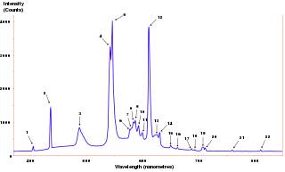
    The power spectrum of a time series describes the distribution of power into frequency components composing that signal. According to Fourier analysis, any physical signal can be decomposed into a number of discrete frequencies, or a spectrum of frequencies over a continuous range. The statistical average of a certain signal or sort of signal as analyzed in terms of its frequency content, is called its spectrum.

    <span class="mw-page-title-main">Theta function</span> Special functions of several complex variables

    In mathematics, theta functions are special functions of several complex variables. They show up in many topics, including Abelian varieties, moduli spaces, quadratic forms, and solitons. As Grassmann algebras, they appear in quantum field theory.

    In mathematics, the Poisson summation formula is an equation that relates the Fourier series coefficients of the periodic summation of a function to values of the function's continuous Fourier transform. Consequently, the periodic summation of a function is completely defined by discrete samples of the original function's Fourier transform. And conversely, the periodic summation of a function's Fourier transform is completely defined by discrete samples of the original function. The Poisson summation formula was discovered by Siméon Denis Poisson and is sometimes called Poisson resummation.

    In control theory and signal processing, a linear, time-invariant system is said to be minimum-phase if the system and its inverse are causal and stable.

    <span class="mw-page-title-main">Cross-correlation</span> Covariance and correlation

    In signal processing, cross-correlation is a measure of similarity of two series as a function of the displacement of one relative to the other. This is also known as a sliding dot product or sliding inner-product. It is commonly used for searching a long signal for a shorter, known feature. It has applications in pattern recognition, single particle analysis, electron tomography, averaging, cryptanalysis, and neurophysiology. The cross-correlation is similar in nature to the convolution of two functions. In an autocorrelation, which is the cross-correlation of a signal with itself, there will always be a peak at a lag of zero, and its size will be the signal energy.

    In pulsed radar and sonar signal processing, an ambiguity function is a two-dimensional function of propagation delay and Doppler frequency , . It represents the distortion of a returned pulse due to the receiver matched filter of the return from a moving target. The ambiguity function is defined by the properties of the pulse and of the filter, and not any particular target scenario.

    In probability theory and statistics, given a stochastic process, the autocovariance is a function that gives the covariance of the process with itself at pairs of time points. Autocovariance is closely related to the autocorrelation of the process in question.

    <span class="mw-page-title-main">Dirac comb</span> Periodic distribution ("function") of "point-mass" Dirac delta sampling

    In mathematics, a Dirac comb is a periodic function with the formula

    In statistics, econometrics, and signal processing, an autoregressive (AR) model is a representation of a type of random process; as such, it is used to describe certain time-varying processes in nature, economics, behavior, etc. The autoregressive model specifies that the output variable depends linearly on its own previous values and on a stochastic term ; thus the model is in the form of a stochastic difference equation. Together with the moving-average (MA) model, it is a special case and key component of the more general autoregressive–moving-average (ARMA) and autoregressive integrated moving average (ARIMA) models of time series, which have a more complicated stochastic structure; it is also a special case of the vector autoregressive model (VAR), which consists of a system of more than one interlocking stochastic difference equation in more than one evolving random variable.

    <span class="mw-page-title-main">Directional statistics</span>

    Directional statistics is the subdiscipline of statistics that deals with directions, axes or rotations in Rn. More generally, directional statistics deals with observations on compact Riemannian manifolds including the Stiefel manifold.

    In applied mathematics, the Wiener–Khinchin theorem or Wiener–Khintchine theorem, also known as the Wiener–Khinchin–Einstein theorem or the Khinchin–Kolmogorov theorem, states that the autocorrelation function of a wide-sense-stationary random process has a spectral decomposition given by the power spectrum of that process.

    <span class="mw-page-title-main">Wigner distribution function</span>

    The Wigner distribution function (WDF) is used in signal processing as a transform in time-frequency analysis.

    In mathematics, a local martingale is a type of stochastic process, satisfying the localized version of the martingale property. Every martingale is a local martingale; every bounded local martingale is a martingale; in particular, every local martingale that is bounded from below is a supermartingale, and every local martingale that is bounded from above is a submartingale; however, in general a local martingale is not a martingale, because its expectation can be distorted by large values of small probability. In particular, a driftless diffusion process is a local martingale, but not necessarily a martingale.

    Stochastic approximation methods are a family of iterative methods typically used for root-finding problems or for optimization problems. The recursive update rules of stochastic approximation methods can be used, among other things, for solving linear systems when the collected data is corrupted by noise, or for approximating extreme values of functions which cannot be computed directly, but only estimated via noisy observations.

    In probability and statistics, the Tweedie distributions are a family of probability distributions which include the purely continuous normal, gamma and inverse Gaussian distributions, the purely discrete scaled Poisson distribution, and the class of compound Poisson–gamma distributions which have positive mass at zero, but are otherwise continuous. Tweedie distributions are a special case of exponential dispersion models and are often used as distributions for generalized linear models.

    Bilinear time–frequency distributions, or quadratic time–frequency distributions, arise in a sub-field of signal analysis and signal processing called time–frequency signal processing, and, in the statistical analysis of time series data. Such methods are used where one needs to deal with a situation where the frequency composition of a signal may be changing over time; this sub-field used to be called time–frequency signal analysis, and is now more often called time–frequency signal processing due to the progress in using these methods to a wide range of signal-processing problems.

    <span class="mw-page-title-main">Rogers–Ramanujan continued fraction</span> Continued fraction closely related to the Rogers–Ramanujan identities

    The Rogers–Ramanujan continued fraction is a continued fraction discovered by Rogers (1894) and independently by Srinivasa Ramanujan, and closely related to the Rogers–Ramanujan identities. It can be evaluated explicitly for a broad class of values of its argument.

    Exponential Tilting (ET), Exponential Twisting, or Exponential Change of Measure (ECM) is a distribution shifting technique used in many parts of mathematics. The different exponential tiltings of a random variable is known as the natural exponential family of .

    References

    1. Gardner, William A.; Antonio Napolitano; Luigi Paura (2006). "Cyclostationarity: Half a century of research". Signal Processing. Elsevier. 86 (4): 639–697. doi:10.1016/j.sigpro.2005.06.016.
    2. 1 2 3 Gardner, William A. (1991). "Two alternative philosophies for estimation of the parameters of time-series". IEEE Trans. Inf. Theory. 37 (1): 216–218. doi:10.1109/18.61145.
    3. 1983 R. A. Boyles and W. A. Gardner. CYCLOERGODIC PROPERTIES OF DISCRETE-PARAMETER NONSTATIONARY STOCHASTIC PROCESSES. IEEE Transactions on Information Theory, Vol. IT-29, No. 1, pp. 105-114.
    4. Kipnis, Alon; Goldsmith, Andrea; Eldar, Yonina (May 2018). "The Distortion Rate Function of Cyclostationary Gaussian Processes". IEEE Transactions on Information Theory. 65 (5): 3810–3824. arXiv: 1505.05586 . doi:10.1109/TIT.2017.2741978. S2CID   5014143.
    5. W. A. Gardner. INTRODUCTION TO RANDOM PROCESSES WITH APPLICATIONS TO SIGNALS AND SYSTEMS. Macmillan, New York, 434 pages, 1985
    6. W. A. Gardner. STATISTICAL SPECTRAL ANALYSIS: A NONPROBABILISTIC THEORY. Prentice-Hall, Englewood Cliffs, NJ, 565 pages, 1987.
    7. W. A. Gardner. STATISTICAL SPECTRAL ANALYSIS: A NONPROBABILISTIC THEORY. Prentice-Hall, Englewood Cliffs, NJ, 565 pages, 1987.
    8. Troutman, B.M. (1979) "Some results in periodic autoregression." Biometrika, 66 (2), 219228
    9. Jones, R.H., Brelsford, W.M. (1967) "Time series with periodic structure." Biometrika, 54, 403410
    10. Pagano, M. (1978) "On periodic and multiple autoregressions." Ann. Stat., 6, 13101317.
    11. W. A. Gardner. STATIONARIZABLE RANDOM PROCESSES. IEEE Transactions on Information Theory, Vol. IT-24, No. 1, pp. 8-22. 1978
    12. W. A. Gardner. STATISTICAL SPECTRAL ANALYSIS: A NONPROBABILISTIC THEORY. Prentice-Hall, Englewood Cliffs, NJ, 565 pages, 1987.
    13. W. A. Gardner. STATISTICAL SPECTRAL ANALYSIS: A NONPROBABILISTIC THEORY. Prentice-Hall, Englewood Cliffs, NJ, 565 pages, 1987.
    14. A. Napolitano, Cyclostationary Processes and Time Series: Theory, Applications, and Generalizations. Academic Press, 2020.
    15. W. A. Gardner. STATISTICALLY INFERRED TIME WARPING: EXTENDING THE CYCLOSTATIONARITY PARADIGM FROM REGULAR TO IRREGULAR STATISTICAL CYCLICITY IN SCIENTIFIC DATA. EURASIP Journal on Advances in Signal Processing volume 2018, Article number: 59. doi: 10.1186/s13634-018-0564-6
    16. A. Napolitano, Cyclostationary Processes and Time Series: Theory, Applications, and Generalizations. Academic Press, 2020.
    17. W. A. Gardner. CYCLOSTATIONARITY IN COMMUNICATIONS AND SIGNAL PROCESSING. Piscataway, NJ: IEEE Press. 504 pages.1984.
    18. W. A. Gardner. SIGNAL INTERCEPTION: A UNIFYING THEORETICAL FRAMEWORK FOR FEATURE DETECTION. IEEE Transactions on Communications, Vol. COM-36, No. 8, pp. 897-906. 1988
    19. Antoni, Jérôme (2009). "Cyclostationarity by examples". Mechanical Systems and Signal Processing. Elsevier. 23 (4): 987–1036. doi:10.1016/j.ymssp.2008.10.010.
    20. 2018 W. A. Gardner. STATISTICALLY INFERRED TIME WARPING: EXTENDING THE CYCLOSTATIONARITY PARADIGM FROM REGULAR TO IRREGULAR STATISTICAL CYCLICITY IN SCIENTIFIC DATA. EURASIP Journal on Advances in Signal Processing volume 2018, Article number: 59. doi: 10.1186/s13634-018-0564-6