
In physics, physical chemistry and engineering, fluid dynamics is a subdiscipline of fluid mechanics that describes the flow of fluids—liquids and gases. It has several subdisciplines, including aerodynamics and hydrodynamics. Fluid dynamics has a wide range of applications, including calculating forces and moments on aircraft, determining the mass flow rate of petroleum through pipelines, predicting weather patterns, understanding nebulae in interstellar space and modelling fission weapon detonation.
In fluid dynamics, turbulence or turbulent flow is fluid motion characterized by chaotic changes in pressure and flow velocity. It is in contrast to a laminar flow, which occurs when a fluid flows in parallel layers, with no disruption between those layers.
Quantum turbulence is the name given to the turbulent flow – the chaotic motion of a fluid at high flow rates – of quantum fluids, such as superfluids. The idea that a form of turbulence might be possible in a superfluid via the quantized vortex lines was first suggested by Richard Feynman. The dynamics of quantum fluids are governed by quantum mechanics, rather than classical physics which govern classical (ordinary) fluids. Some examples of quantum fluids include superfluid helium, Bose–Einstein condensates (BECs), polariton condensates, and nuclear pasta theorized to exist inside neutron stars. Quantum fluids exist at temperatures below the critical temperature at which Bose-Einstein condensation takes place.

A scintillometer is a scientific device used to measure turbulent fluctuations of the refractive index of air caused by variations in temperature, humidity, and pressure. It consists of an optical or radio wave transmitter and a receiver at opposite ends of an atmospheric propagation path. The receiver detects and evaluates the intensity fluctuations of the transmitted signal, called scintillation.

Large eddy simulation (LES) is a mathematical model for turbulence used in computational fluid dynamics. It was initially proposed in 1963 by Joseph Smagorinsky to simulate atmospheric air currents, and first explored by Deardorff (1970). LES is currently applied in a wide variety of engineering applications, including combustion, acoustics, and simulations of the atmospheric boundary layer.
In fluid dynamics, the Reynolds stress is the component of the total stress tensor in a fluid obtained from the averaging operation over the Navier–Stokes equations to account for turbulent fluctuations in fluid momentum.

In fluid dynamics, Kolmogorov microscales are the smallest scales in the turbulent flow of fluids. At the Kolmogorov scale, viscosity dominates and the turbulence kinetic energy is dissipated into thermal energy. They are defined by
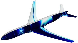
In fluid dynamics, turbulence modeling is the construction and use of a mathematical model to predict the effects of turbulence. Turbulent flows are commonplace in most real-life scenarios, including the flow of blood through the cardiovascular system, the airflow over an aircraft wing, the re-entry of space vehicles, besides others. In spite of decades of research, there is no analytical theory to predict the evolution of these turbulent flows. The equations governing turbulent flows can only be solved directly for simple cases of flow. For most real-life turbulent flows, CFD simulations use turbulent models to predict the evolution of turbulence. These turbulence models are simplified constitutive equations that predict the statistical evolution of turbulent flows.
A direct numerical simulation (DNS) is a simulation in computational fluid dynamics (CFD) in which the Navier–Stokes equations are numerically solved without any turbulence model. This means that the whole range of spatial and temporal scales of the turbulence must be resolved. All the spatial scales of the turbulence must be resolved in the computational mesh, from the smallest dissipative scales, up to the integral scale , associated with the motions containing most of the kinetic energy. The Kolmogorov scale, , is given by
In fluid dynamics, turbulence kinetic energy (TKE) is the mean kinetic energy per unit mass associated with eddies in turbulent flow. Physically, the turbulence kinetic energy is characterised by measured root-mean-square (RMS) velocity fluctuations. In the Reynolds-averaged Navier Stokes equations, the turbulence kinetic energy can be calculated based on the closure method, i.e. a turbulence model.
In continuum mechanics, wave turbulence is a set of nonlinear waves deviated far from thermal equilibrium. Such a state is usually accompanied by dissipation. It is either decaying turbulence or requires an external source of energy to sustain it. Examples are waves on a fluid surface excited by winds or ships, and waves in plasma excited by electromagnetic waves etc.
Robert Harry Kraichnan, a resident of Santa Fe, New Mexico, was an American theoretical physicist best known for his work on the theory of fluid turbulence.
In fluid dynamics, a Tollmien–Schlichting wave is a streamwise unstable wave which arises in a bounded shear flow. It is one of the more common methods by which a laminar bounded shear flow transitions to turbulence. The waves are initiated when some disturbance interacts with leading edge roughness in a process known as receptivity. These waves are slowly amplified as they move downstream until they may eventually grow large enough that nonlinearities take over and the flow transitions to turbulence.
In fluid dynamics, the Taylor microscale, which is sometimes called the turbulence length scale, is a length scale used to characterize a turbulent fluid flow. This microscale is named after Geoffrey Ingram Taylor. The Taylor microscale is the intermediate length scale at which fluid viscosity significantly affects the dynamics of turbulent eddies in the flow. This length scale is traditionally applied to turbulent flow which can be characterized by a Kolmogorov spectrum of velocity fluctuations. In such a flow, length scales which are larger than the Taylor microscale are not strongly affected by viscosity. These larger length scales in the flow are generally referred to as the inertial range. Below the Taylor microscale the turbulent motions are subject to strong viscous forces and kinetic energy is dissipated into heat. These shorter length scale motions are generally termed the dissipation range.

In fluid mechanics, the Reynolds number is a dimensionless quantity that helps predict fluid flow patterns in different situations by measuring the ratio between inertial and viscous forces. At low Reynolds numbers, flows tend to be dominated by laminar (sheet-like) flow, while at high Reynolds numbers, flows tend to be turbulent. The turbulence results from differences in the fluid's speed and direction, which may sometimes intersect or even move counter to the overall direction of the flow. These eddy currents begin to churn the flow, using up energy in the process, which for liquids increases the chances of cavitation.
In fluid and molecular dynamics, the Batchelor scale, determined by George Batchelor (1959), describes the size of a droplet of fluid that will diffuse in the same time it takes the energy in an eddy of size η to dissipate. The Batchelor scale can be determined by:
Magnetohydrodynamic turbulence concerns the chaotic regimes of magnetofluid flow at high Reynolds number. Magnetohydrodynamics (MHD) deals with what is a quasi-neutral fluid with very high conductivity. The fluid approximation implies that the focus is on macro length-and-time scales which are much larger than the collision length and collision time respectively.
K-epsilon (k-ε) turbulence model is the most common model used in computational fluid dynamics (CFD) to simulate mean flow characteristics for turbulent flow conditions. It is a two equation model that gives a general description of turbulence by means of two transport equations. The original impetus for the K-epsilon model was to improve the mixing-length model, as well as to find an alternative to algebraically prescribing turbulent length scales in moderate to high complexity flows.
Reynolds stress equation model (RSM), also referred to as second moment closures are the most complete classical turbulence model. In these models, the eddy-viscosity hypothesis is avoided and the individual components of the Reynolds stress tensor are directly computed. These models use the exact Reynolds stress transport equation for their formulation. They account for the directional effects of the Reynolds stresses and the complex interactions in turbulent flows. Reynolds stress models offer significantly better accuracy than eddy-viscosity based turbulence models, while being computationally cheaper than Direct Numerical Simulations (DNS) and Large Eddy Simulations.
Multiscale turbulence is a class of turbulent flows in which the chaotic motion of the fluid is forced at different length and/or time scales. This is usually achieved by immersing in a moving fluid a body with a multiscale, often fractal-like, arrangement of length scales. This arrangement of scales can be either passive or active


