Entrance length (fluid dynamics)

Last updated

In fluid dynamics, the entrance length is the distance a flow travels after entering a pipe before the flow becomes fully developed. [1] Entrance length refers to the length of the entry region, the area following the pipe entrance where effects originating from the interior wall of the pipe propagate into the flow as an expanding boundary layer. When the boundary layer expands to fill the entire pipe, the developing flow becomes a fully developed flow, where flow characteristics no longer change with increased distance along the pipe. Many different entrance lengths exist to describe a variety of flow conditions. Hydrodynamic entrance length describes the formation of a velocity profile caused by viscous forces propagating from the pipe wall. Thermal entrance length describes the formation of a temperature profile. [2] Awareness of entrance length may be necessary for the effective placement of instrumentation, such as fluid flow meters. [3]

Contents

Hydrodynamic entrance length

The hydrodynamic entrance region refers to the area of a pipe where fluid entering a pipe develops a velocity profile due to viscous forces propagating from the interior wall of a pipe. [1] This region is characterized by a non-uniform flow. [1] The fluid enters a pipe at a uniform velocity, then fluid particles in the layer in contact with the surface of the pipe come to a complete stop due to the no-slip condition. Due to viscous forces within the fluid, the layer in contact with the pipe surface resists the motion of adjacent layers and slows adjacent layers of fluid down gradually, forming a velocity profile. [4] For the conservation of mass to hold true, the velocity of layers of the fluid in the center of the pipe increases to compensate for the reduced velocities of the layers of fluid near the pipe surface. This develops a velocity gradient across the cross-section of the pipe. [5]

Boundary layer

The layer in which the shearing viscous forces are significant, is called the boundary layer. [6] This boundary layer is a hypothetical concept. It divides the flow in pipe into two regions: [6]

  1. Boundary layer region: The region in which viscous effects and the velocity changes are significant. [6]
  2. The irrotational (core) flow region: The region in which viscous effects and velocity changes are negligible, also known as the inviscid core. [2]

When the fluid just enters the pipe, the thickness of the boundary layer gradually increases from zero moving in the direction of fluid flow and eventually reaches the pipe center and fills the entire pipe. This region from the entrance of the pipe to the point where the boundary layer covers the entire pipe is termed as the hydrodynamic entrance region and the length of the pipe in this region is termed as the hydrodynamic entry length. In this region, the velocity profile develops and thus the flow is called the hydrodynamically developing flow. After this region, the velocity profile is fully developed and continues unchanged. This region is called the hydrodynamically fully developed region. But this is not the fully developed fluid flow until the normalized temperature profile also becomes constant. [6]

In case of laminar flow, the velocity profile in the fully developed region is parabolic but in the case of turbulent flow it gets a little flatter due to vigorous mixing in radial direction and eddy motion.


The velocity profile remains unchanged in the fully developed region.

Hydrodynamic Fully Developed velocity profile Laminar Flow :

[6]

where is in the flow direction.

The developing velocity profile of a fluid entering a pipe. Development of fluid flow in the entrance region of a pipe.jpg
The developing velocity profile of a fluid entering a pipe.

Shear stress

In the hydrodynamic entrance region, the wall shear stress, , is highest at the pipe inlet, where the boundary layer thickness is the smallest. Shear stress decreases along the flow direction. [6] That is why the pressure drop is highest in the entrance region of a pipe, which increases the average friction factor for the whole pipe. This increase in the friction factor is negligible for long pipes. [6] In a fully developed region, the pressure gradient and the shear stress in flow are in balance. [6]

Variation of Shear Stress with distance from the entry point. Variation of Shear Stress with distance from the entry point.png
Variation of Shear Stress with distance from the entry point.

Calculating hydrodynamic entrance length

The length of the hydrodynamic entry region along the pipe is called the hydrodynamic entry length. It is a function of Reynolds number of the flow. In case of laminar flow, this length is given by:

[2]

where is the Reynolds number and is the diameter of the pipe.
But in the case of turbulent flow,

[8]

Thus, the entry length in turbulent flow is much shorter as compared to laminar one. In most practical engineering applications, this entrance effect becomes insignificant beyond a pipe length of 10 times the diameter and hence it is approximated to be:

[6]
Other authors give much longer entrance length, e.g.

Entry length for pipes with non-circular cross-sections

In the case of a non-circular cross-section of a pipe, the same formula can be used to find the entry length with a little modification. A new parameter “hydraulic diameter” relates the flow in non-circular pipe to that of circular pipe flow. This is valid as long as the cross-sectional area shape is not too exaggerated. Hydraulic Diameter is defined as:

[6]

where is the area of cross-section and is the Perimeter of the wet part of the pipe

Average velocity of fully developed flow

By doing a force balance on a small volume element in the fully developed flow region in the pipe (Laminar Flow), we get velocity as function of radius only i.e. it does not depend upon the axial distance from the entry point. [6] The velocity as the function of radius comes out to be:

[6]
where is constant.

By definition of average velocity is given by

where is cross-sectional area.

Thus,

[6]

For fully developed flow, the maximum velocity will be at .
Thus,

[6]

Thermal entrance length

The thermal entrance length is the distance for incoming flow in a pipe to form a temperature profile with a stable shape. The shape of the fully developed temperature profile is determined by temperature and heat flux conditions along the inside wall of the pipe, as well as fluid properties. [2]

Overview

Fully developed heat flow in a pipe can be considered in the following situation. If the wall of the pipe is constantly heated or cooled so that the heat flux from the wall to the fluid via convection is a fixed value, then the bulk temperature of the fluid steadily increases or decreases respectively at a fixed rate along the flow direction.

An example can be a pipe entirely covered by an electrical heating pad with the flow being introduced after a uniform heat flux from the pad is achieved. At some distance away from the entrance of the fluid, fully developed heat flow is achieved when the heat transfer coefficient of the fluid becomes constant and the temperature profile has the same shape along the flow. [11] This distance is defined as the thermal entrance length, which is important for engineers to design efficient heat transfer processes.

Laminar flow

For laminar flow, the thermal entrance length is a function of pipe diameter and the dimensionless Reynolds number and Prandtl number. [2]

[2]

where

The Prandtl number modifies the hydrodynamic entrance length to determine thermal entrance length. The Prandtl number is the dimensionless number for the ratio of momentum diffusivity to thermal diffusivity. [5] The thermal entrance length for a fluid with a Prandtl number greater than one will be longer than the hydrodynamic entrance length, and shorter if the Prandtl number is less than one. For example, molten sodium has a low Prandtl number of 0.004, [12] so the thermal entrance length will be significantly shorter than the hydraulic entrance length.

For turbulent flows, thermal entrance length may be approximated solely based on pipe diameter. [2]

[2]

where

Heat transfer

The development of the temperature profile in the flow is driven by heat transfer determined conditions on the inside surface of the pipe and the fluid. [2] Heat transfer may be a result of a constant heat flux or constant surface temperature. Constant heat flux may be caused by joule heating from a heat source, like heat tape, wrapped around the pipe. [13] Constant temperature conditions may be produced by a phase transition, such as condensation of saturated steam on a pipe surface. [14]

Newtons law of cooling describes convection, the main form of heat transport between the fluid and the pipe:

[2]

where

Constant surface heat flux result in becoming a constant as the flow develops and constant surface temperature results in approaching zero. [2]

Thermally fully developed flow

Unlike hydrodynamic developed flow, a constant profile shape is used to define thermally fully developed flow because temperature continually approaches ambient temperature. [2] Dimensionless analysis of change in profile shape defines when a flow is thermally fully developed.

Requirement for thermally fully developed flow:

[2]

Thermally developed flow results in reduced heat transfer compared to developing flow because the difference between the surface temperature of the pipe and the mean temperature of the flow is greater than the temperature difference between surface temperature of the pipe and the temperature of the fluid near the pipe boundary. [2]

Concentration entrance length

The concentration entrance length describes the length needed for the concentration profile in a flow to be fully developed. The concentration entrance length can be determined by relating it to the hydrodynamic entrance length with the Schmidt number or by experimental techniques. [15] The Schmidt number describes the ratio of momentum diffusivity to mass diffusivity. [2]

[2]

where

Applications

Understanding the entrance length is important for the design and analysis of flow systems. The entrance region will have different velocity, temperature, and other profiles than exist in the fully developed region of the pipe.

Flow meters

Illustration of a Venturi flow meter, an example of a differential-pressure flow meter. VenturiTubeScheme.png
Illustration of a Venturi flow meter, an example of a differential-pressure flow meter.

Many types of flow instrumentation, such as flow meters, require a fully developed flow to function properly. [3] Common flow meters, including vortex flow meters and differential-pressure flow meters, require hydrodynamically fully developed flow. Hydraulically fully developed flow is commonly achieved by having long, straight sections of pipe before the flow meter. Alternatively, flow conditioners and straightening devices may be used to produce the desired flow. [17]

Wind tunnels

Wind tunnels use an inviscid flow of air to test the aerodynamics of an object. Flow straighteners, which consist of many parallel ducts which limit turbulence, are used to produce inviscid flow. [18] Entrance length must be considered in the design of wind tunnels, because the object being tested must be located in the irrotational flow region, between the flow straighteners and the entrance length. [19]

Exit length

Similar to the development of flow at the entrance of the pipe, the flow velocity profile changes before the exit of a pipe. The exit length is much shorter than the entrance length, and is not significant at moderate to high Reynolds numbers. [20]

Hydraulic exit length for laminar flows may be approximated as: [20]

where

See also

Related Research Articles

<span class="mw-page-title-main">Fluid dynamics</span> Aspects of fluid mechanics involving flow

In physics, physical chemistry and engineering, fluid dynamics is a subdiscipline of fluid mechanics that describes the flow of fluids—liquids and gases. It has several subdisciplines, including aerodynamics and hydrodynamics. Fluid dynamics has a wide range of applications, including calculating forces and moments on aircraft, determining the mass flow rate of petroleum through pipelines, predicting weather patterns, understanding nebulae in interstellar space and modelling fission weapon detonation.

<span class="mw-page-title-main">Laminar flow</span> Flow where fluid particles follow smooth paths in layers

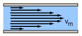
Laminar flow is the property of fluid particles in fluid dynamics to follow smooth paths in layers, with each layer moving smoothly past the adjacent layers with little or no mixing. At low velocities, the fluid tends to flow without lateral mixing, and adjacent layers slide past one another smoothly. There are no cross-currents perpendicular to the direction of flow, nor eddies or swirls of fluids. In laminar flow, the motion of the particles of the fluid is very orderly with particles close to a solid surface moving in straight lines parallel to that surface. Laminar flow is a flow regime characterized by high momentum diffusion and low momentum convection.

The Prandtl number (Pr) or Prandtl group is a dimensionless number, named after the German physicist Ludwig Prandtl, defined as the ratio of momentum diffusivity to thermal diffusivity. The Prandtl number is given as:

In thermal fluid dynamics, the Nusselt number is the ratio of total heat transfer to conductive heat transfer at a boundary in a fluid. Total heat transfer combines conduction and convection. Convection includes both advection and diffusion (conduction). The conductive component is measured under the same conditions as the convective but for a hypothetically motionless fluid. It is a dimensionless number, closely related to the fluid's Rayleigh number.

In fluid mechanics, the Rayleigh number (Ra, after Lord Rayleigh) for a fluid is a dimensionless number associated with buoyancy-driven flow, also known as free (or natural) convection. It characterises the fluid's flow regime: a value in a certain lower range denotes laminar flow; a value in a higher range, turbulent flow. Below a certain critical value, there is no fluid motion and heat transfer is by conduction rather than convection. For most engineering purposes, the Rayleigh number is large, somewhere around 106 to 108.

In fluid dynamics, the Darcy–Weisbach equation is an empirical equation that relates the head loss, or pressure loss, due to friction along a given length of pipe to the average velocity of the fluid flow for an incompressible fluid. The equation is named after Henry Darcy and Julius Weisbach. Currently, there is no formula more accurate or universally applicable than the Darcy-Weisbach supplemented by the Moody diagram or Colebrook equation.

<span class="mw-page-title-main">Boundary layer</span> Layer of fluid in the immediate vicinity of a bounding surface

In physics and fluid mechanics, a boundary layer is the thin layer of fluid in the immediate vicinity of a bounding surface formed by the fluid flowing along the surface. The fluid's interaction with the wall induces a no-slip boundary condition. The flow velocity then monotonically increases above the surface until it returns to the bulk flow velocity. The thin layer consisting of fluid whose velocity has not yet returned to the bulk flow velocity is called the velocity boundary layer.

In thermodynamics, the heat transfer coefficient or film coefficient, or film effectiveness, is the proportionality constant between the heat flux and the thermodynamic driving force for the flow of heat. It is used in calculating the heat transfer, typically by convection or phase transition between a fluid and a solid. The heat transfer coefficient has SI units in watts per square meter per kelvin (W/m²K).

<span class="mw-page-title-main">Plug flow</span> Simple model of fluid flow in a pipe

In fluid mechanics, plug flow is a simple model of the velocity profile of a fluid flowing in a pipe. In plug flow, the velocity of the fluid is assumed to be constant across any cross-section of the pipe perpendicular to the axis of the pipe. The plug flow model assumes there is no boundary layer adjacent to the inner wall of the pipe.

In fluid dynamics, the Schmidt number of a fluid is a dimensionless number defined as the ratio of momentum diffusivity and mass diffusivity, and it is used to characterize fluid flows in which there are simultaneous momentum and mass diffusion convection processes. It was named after German engineer Ernst Heinrich Wilhelm Schmidt (1892–1975).

The Stanton number, St, is a dimensionless number that measures the ratio of heat transferred into a fluid to the thermal capacity of fluid. The Stanton number is named after Thomas Stanton (engineer) (1865–1931). It is used to characterize heat transfer in forced convection flows.

<span class="mw-page-title-main">Law of the wall</span> Relation of flow speed to wall distance

In fluid dynamics, the law of the wall states that the average velocity of a turbulent flow at a certain point is proportional to the logarithm of the distance from that point to the "wall", or the boundary of the fluid region. This law of the wall was first published in 1930 by Hungarian-American mathematician, aerospace engineer, and physicist Theodore von Kármán. It is only technically applicable to parts of the flow that are close to the wall, though it is a good approximation for the entire velocity profile of natural streams.

This page describes some of the parameters used to characterize the thickness and shape of boundary layers formed by fluid flowing along a solid surface. The defining characteristic of boundary layer flow is that at the solid walls, the fluid's velocity is reduced to zero. The boundary layer refers to the thin transition layer between the wall and the bulk fluid flow. The boundary layer concept was originally developed by Ludwig Prandtl and is broadly classified into two types, bounded and unbounded. The differentiating property between bounded and unbounded boundary layers is whether the boundary layer is being substantially influenced by more than one wall. Each of the main types has a laminar, transitional, and turbulent sub-type. The two types of boundary layers use similar methods to describe the thickness and shape of the transition region with a couple of exceptions detailed in the Unbounded Boundary Layer Section. The characterizations detailed below consider steady flow but is easily extended to unsteady flow.

The Reynolds Analogy is popularly known to relate turbulent momentum and heat transfer. That is because in a turbulent flow the transport of momentum and the transport of heat largely depends on the same turbulent eddies: the velocity and the temperature profiles have the same shape.

The turbulent Prandtl number (Prt) is a non-dimensional term defined as the ratio between the momentum eddy diffusivity and the heat transfer eddy diffusivity. It is useful for solving the heat transfer problem of turbulent boundary layer flows. The simplest model for Prt is the Reynolds analogy, which yields a turbulent Prandtl number of 1. From experimental data, Prt has an average value of 0.85, but ranges from 0.7 to 0.9 depending on the Prandtl number of the fluid in question.

In nonideal fluid dynamics, the Hagen–Poiseuille equation, also known as the Hagen–Poiseuille law, Poiseuille law or Poiseuille equation, is a physical law that gives the pressure drop in an incompressible and Newtonian fluid in laminar flow flowing through a long cylindrical pipe of constant cross section. It can be successfully applied to air flow in lung alveoli, or the flow through a drinking straw or through a hypodermic needle. It was experimentally derived independently by Jean Léonard Marie Poiseuille in 1838 and Gotthilf Heinrich Ludwig Hagen, and published by Hagen in 1839 and then by Poiseuille in 1840–41 and 1846. The theoretical justification of the Poiseuille law was given by George Stokes in 1845.

<span class="mw-page-title-main">Reynolds number</span> Ratio of inertial to viscous forces acting on a liquid

In fluid dynamics, the Reynolds number is a dimensionless quantity that helps predict fluid flow patterns in different situations by measuring the ratio between inertial and viscous forces. At low Reynolds numbers, flows tend to be dominated by laminar (sheet-like) flow, while at high Reynolds numbers, flows tend to be turbulent. The turbulence results from differences in the fluid's speed and direction, which may sometimes intersect or even move counter to the overall direction of the flow. These eddy currents begin to churn the flow, using up energy in the process, which for liquids increases the chances of cavitation.

In engineering, physics, and chemistry, the study of transport phenomena concerns the exchange of mass, energy, charge, momentum and angular momentum between observed and studied systems. While it draws from fields as diverse as continuum mechanics and thermodynamics, it places a heavy emphasis on the commonalities between the topics covered. Mass, momentum, and heat transport all share a very similar mathematical framework, and the parallels between them are exploited in the study of transport phenomena to draw deep mathematical connections that often provide very useful tools in the analysis of one field that are directly derived from the others.

Skin friction drag is a type of aerodynamic or hydrodynamic drag, which is resistant force exerted on an object moving in a fluid. Skin friction drag is caused by the viscosity of fluids and is developed from laminar drag to turbulent drag as a fluid moves on the surface of an object. Skin friction drag is generally expressed in terms of the Reynolds number, which is the ratio between inertial force and viscous force.

<span class="mw-page-title-main">Thermal boundary layer thickness and shape</span>

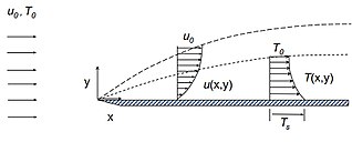
This page describes some parameters used to characterize the properties of the thermal boundary layer formed by a heated fluid moving along a heated wall. In many ways, the thermal boundary layer description parallels the velocity (momentum) boundary layer description first conceptualized by Ludwig Prandtl. Consider a fluid of uniform temperature and velocity impinging onto a stationary plate uniformly heated to a temperature . Assume the flow and the plate are semi-infinite in the positive/negative direction perpendicular to the plane. As the fluid flows along the wall, the fluid at the wall surface satisfies a no-slip boundary condition and has zero velocity, but as you move away from the wall, the velocity of the flow asymptotically approaches the free stream velocity . The temperature at the solid wall is and gradually changes to as one moves toward the free stream of the fluid. It is impossible to define a sharp point at which the thermal boundary layer fluid or the velocity boundary layer fluid becomes the free stream, yet these layers have a well-defined characteristic thickness given by and . The parameters below provide a useful definition of this characteristic, measurable thickness for the thermal boundary layer. Also included in this boundary layer description are some parameters useful in describing the shape of the thermal boundary layer.

References

  1. 1 2 3 ES162_08_Notes02a_Flow_In_Pipes_Changtamu.Pdf. 1st ed. Cambridge: J. R. Rice, 2017. Print.
  2. 1 2 3 4 5 6 7 8 9 10 11 12 13 14 15 16 Bergman, T.L.; Incropera, Frank P. (2011-01-01). Fundamentals of heat and mass transfer. Wiley. ISBN   9780470501979. OCLC   713621645.
  3. 1 2 Marghitu, Dan (2001). Mechanical Engineer's Handbook. Elsevier. pp. Section 402.1 Page 6 via Knovel.
  4. Stewart, Warren E.; Lightfoot, Edwin N. (2007-01-01). Transport phenomena. J. Wiley. ISBN   978-0471410775. OCLC   77079936.
  5. 1 2 White, Frank M. (2006-01-01). Viscous fluid flow. McGraw-Hill Higher Education. ISBN   978-0072402315. OCLC   693819619.
  6. 1 2 3 4 5 6 7 8 9 10 11 12 13 14 Cimbala, Yungas A.; Çengel, John M. (2006). Fluid mechanics : fundamentals and applications (1st ed.). Boston: McGraw-Hill Higher Education. pp.  321, 322, 323, 324, 325, 326, 327, 328, 329. ISBN   978-0072472363.
  7. 1 2 Cimbala, John M. (2006-01-01). Fluid mechanics : fundamentals and applications. McGraw-Hill Higher Education. ISBN   978-0072472363. OCLC   834846067.
  8. Çengel, Yunus A. (2018). Fluid mechanics : fundamentals and applications. John M. Cimbala (Fourth ed.). New York, NY. ISBN   978-1-259-69653-4. OCLC   958355753.{{cite book}}: CS1 maint: location missing publisher (link)
  9. Nikuradse, J., Gesetzmäßigkeiten der turbulenten Strömung in glatten Rohren, Forschung auf dem Gebiet des Ingenieurwesens, 3, 1932, 1–36, (Translated in NASA TT F-10, 359,1966.
  10. Lien, K.; et al. (2004). "The Entrance Length for Fully Developed Turbulent Channel Flow" (PDF). 15th Australasian Fluid Mechanics Conference.
  11. Mills, A. F.(1999)Heat Transfer. 2nd Ed. Prentice Hall, Upper Saddle River, New Jersey
  12. Richardson, J. F.; Backhurst, J. R.; Harker, J. H. (1995-01-01). Fluid flow, heat transfer and mass transfer. Butterworth-Heinemann. ISBN   9780750644440. OCLC   505103987.
  13. "G1408 Electric Heat Cable for Farm and Home Use | University of Missouri Extension". extension.missouri.edu. Archived from the original on 2017-03-12. Retrieved 2017-03-11.
  14. Ashrae (2016-01-01). HVAC Systems and Equipment 2016 SI Edition: Heating, Ventilating, and Air-Conditioning Systems and Equipment. Amer Society of Heating. ISBN   9781939200273. OCLC   947795042.
  15. J. Electrochem. Soc. 160 (2013) E5-E11; doi:10.1149/2.015302jes
  16. Formanavt (2009-02-07), Русский: Устройство трубы Вентури , retrieved 2017-03-11
  17. "Flowmeter piping requirements | Flow Control Network". Flow Control Network. 2010-09-26. Retrieved 2017-03-11.
  18. Farell, C., Youssef, S., 1996. Experiments on turbulence management using screens and honeycombs. ASME J. Fluids Eng.
  19. "chapt3". history.nasa.gov. Retrieved 2017-03-11.
  20. 1 2 Perry, Robert H., Don W.; Green (2008-01-01). Perry's chemical engineers' handbook. McGraw-Hill. ISBN   978-0071593137. OCLC   72470708.