
The Navier–Stokes equations are partial differential equations which describe the motion of viscous fluid substances. They were named after French engineer and physicist Claude-Louis Navier and the Irish physicist and mathematician George Gabriel Stokes. They were developed over several decades of progressively building the theories, from 1822 (Navier) to 1842–1850 (Stokes).

Noether's theorem states that every continuous symmetry of the action of a physical system with conservative forces has a corresponding conservation law. This is the first of two theorems proven by mathematician Emmy Noether in 1915 and published in 1918. The action of a physical system is the integral over time of a Lagrangian function, from which the system's behavior can be determined by the principle of least action. This theorem only applies to continuous and smooth symmetries of physical space.
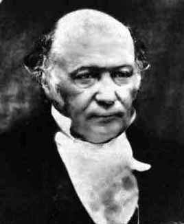
In physics, Hamiltonian mechanics is a reformulation of Lagrangian mechanics that emerged in 1833. Introduced by Sir William Rowan Hamilton, Hamiltonian mechanics replaces (generalized) velocities used in Lagrangian mechanics with (generalized) momenta. Both theories provide interpretations of classical mechanics and describe the same physical phenomena.
In fluid dynamics, Stokes' law is an empirical law for the frictional force – also called drag force – exerted on spherical objects with very small Reynolds numbers in a viscous fluid. It was derived by George Gabriel Stokes in 1851 by solving the Stokes flow limit for small Reynolds numbers of the Navier–Stokes equations.
In mathematical analysis, a function of bounded variation, also known as BV function, is a real-valued function whose total variation is bounded (finite): the graph of a function having this property is well behaved in a precise sense. For a continuous function of a single variable, being of bounded variation means that the distance along the direction of the y-axis, neglecting the contribution of motion along x-axis, traveled by a point moving along the graph has a finite value. For a continuous function of several variables, the meaning of the definition is the same, except for the fact that the continuous path to be considered cannot be the whole graph of the given function, but can be every intersection of the graph itself with a hyperplane parallel to a fixed x-axis and to the y-axis.
In probability theory and related fields, Malliavin calculus is a set of mathematical techniques and ideas that extend the mathematical field of calculus of variations from deterministic functions to stochastic processes. In particular, it allows the computation of derivatives of random variables. Malliavin calculus is also called the stochastic calculus of variations. P. Malliavin first initiated the calculus on infinite dimensional space. Then, the significant contributors such as S. Kusuoka, D. Stroock, J-M. Bismut, Shinzo Watanabe, I. Shigekawa, and so on finally completed the foundations.
A stochastic differential equation (SDE) is a differential equation in which one or more of the terms is a stochastic process, resulting in a solution which is also a stochastic process. SDEs have many applications throughout pure mathematics and are used to model various behaviours of stochastic models such as stock prices, random growth models or physical systems that are subjected to thermal fluctuations.

In quantum field theory, the Lehmann–Symanzik–Zimmermann (LSZ) reduction formula is a method to calculate S-matrix elements from the time-ordered correlation functions of a quantum field theory. It is a step of the path that starts from the Lagrangian of some quantum field theory and leads to prediction of measurable quantities. It is named after the three German physicists Harry Lehmann, Kurt Symanzik and Wolfhart Zimmermann.

Stokes flow, also named creeping flow or creeping motion, is a type of fluid flow where advective inertial forces are small compared with viscous forces. The Reynolds number is low, i.e. . This is a typical situation in flows where the fluid velocities are very slow, the viscosities are very large, or the length-scales of the flow are very small. Creeping flow was first studied to understand lubrication. In nature, this type of flow occurs in the swimming of microorganisms and sperm. In technology, it occurs in paint, MEMS devices, and in the flow of viscous polymers generally.
In mathematics, a locally integrable function is a function which is integrable on every compact subset of its domain of definition. The importance of such functions lies in the fact that their function space is similar to Lp spaces, but its members are not required to satisfy any growth restriction on their behavior at the boundary of their domain : in other words, locally integrable functions can grow arbitrarily fast at the domain boundary, but are still manageable in a way similar to ordinary integrable functions.
In the mathematical field of dynamical systems, a random dynamical system is a dynamical system in which the equations of motion have an element of randomness to them. Random dynamical systems are characterized by a state space S, a set of maps from S into itself that can be thought of as the set of all possible equations of motion, and a probability distribution Q on the set that represents the random choice of map. Motion in a random dynamical system can be informally thought of as a state evolving according to a succession of maps randomly chosen according to the distribution Q.
In mathematics, the trace operator extends the notion of the restriction of a function to the boundary of its domain to "generalized" functions in a Sobolev space. This is particularly important for the study of partial differential equations with prescribed boundary conditions, where weak solutions may not be regular enough to satisfy the boundary conditions in the classical sense of functions.
In mathematics, and especially gauge theory, Seiberg–Witten invariants are invariants of compact smooth oriented 4-manifolds introduced by Edward Witten, using the Seiberg–Witten theory studied by Nathan Seiberg and Witten during their investigations of Seiberg–Witten gauge theory.
Lagrangian field theory is a formalism in classical field theory. It is the field-theoretic analogue of Lagrangian mechanics. Lagrangian mechanics is used to analyze the motion of a system of discrete particles each with a finite number of degrees of freedom. Lagrangian field theory applies to continua and fields, which have an infinite number of degrees of freedom.
In machine learning, the kernel embedding of distributions comprises a class of nonparametric methods in which a probability distribution is represented as an element of a reproducing kernel Hilbert space (RKHS). A generalization of the individual data-point feature mapping done in classical kernel methods, the embedding of distributions into infinite-dimensional feature spaces can preserve all of the statistical features of arbitrary distributions, while allowing one to compare and manipulate distributions using Hilbert space operations such as inner products, distances, projections, linear transformations, and spectral analysis. This learning framework is very general and can be applied to distributions over any space on which a sensible kernel function may be defined. For example, various kernels have been proposed for learning from data which are: vectors in , discrete classes/categories, strings, graphs/networks, images, time series, manifolds, dynamical systems, and other structured objects. The theory behind kernel embeddings of distributions has been primarily developed by Alex Smola, Le Song , Arthur Gretton, and Bernhard Schölkopf. A review of recent works on kernel embedding of distributions can be found in.
The Leray projection, named after Jean Leray, is a linear operator used in the theory of partial differential equations, specifically in the fields of fluid dynamics. Informally, it can be seen as the projection on the divergence-free vector fields. It is used in particular to eliminate both the pressure term and the divergence-free term in the Stokes equations and Navier–Stokes equations.
The variational multiscale method (VMS) is a technique used for deriving models and numerical methods for multiscale phenomena. The VMS framework has been mainly applied to design stabilized finite element methods in which stability of the standard Galerkin method is not ensured both in terms of singular perturbation and of compatibility conditions with the finite element spaces.
The streamline upwind Petrov–Galerkin pressure-stabilizing Petrov–Galerkin formulation for incompressible Navier–Stokes equations can be used for finite element computations of high Reynolds number incompressible flow using equal order of finite element space by introducing additional stabilization terms in the Navier–Stokes Galerkin formulation.
The Bueno-Orovio–Cherry–Fenton model, also simply called Bueno-Orovio model, is a minimal ionic model for human ventricular cells. It belongs to the category of phenomenological models, because of its characteristic of describing the electrophysiological behaviour of cardiac muscle cells without taking into account in a detailed way the underlying physiology and the specific mechanisms occurring inside the cells.
In mathematics, and especially differential geometry and mathematical physics, gauge theory is the general study of connections on vector bundles, principal bundles, and fibre bundles. Gauge theory in mathematics should not be confused with the closely related concept of a gauge theory in physics, which is a field theory which admits gauge symmetry. In mathematics theory means a mathematical theory, encapsulating the general study of a collection of concepts or phenomena, whereas in the physical sense a gauge theory is a mathematical model of some natural phenomenon.


