
In probability theory and statistics, the exponential distribution or negative exponential distribution is the probability distribution of the distance between events in a Poisson point process, i.e., a process in which events occur continuously and independently at a constant average rate; the distance parameter could be any meaningful mono-dimensional measure of the process, such as time between production errors, or length along a roll of fabric in the weaving manufacturing process. It is a particular case of the gamma distribution. It is the continuous analogue of the geometric distribution, and it has the key property of being memoryless. In addition to being used for the analysis of Poisson point processes it is found in various other contexts.

The Pareto distribution, named after the Italian civil engineer, economist, and sociologist Vilfredo Pareto, is a power-law probability distribution that is used in description of social, quality control, scientific, geophysical, actuarial, and many other types of observable phenomena; the principle originally applied to describing the distribution of wealth in a society, fitting the trend that a large portion of wealth is held by a small fraction of the population. The Pareto principle or "80-20 rule" stating that 80% of outcomes are due to 20% of causes was named in honour of Pareto, but the concepts are distinct, and only Pareto distributions with shape value of log45 ≈ 1.16 precisely reflect it. Empirical observation has shown that this 80-20 distribution fits a wide range of cases, including natural phenomena and human activities.

In probability theory and statistics, the Weibull distribution is a continuous probability distribution. It models a broad range of random variables, largely in the nature of a time to failure or time between events. Examples are maximum one-day rainfalls and the time a user spends on a web page.
In mathematics, the Hodge star operator or Hodge star is a linear map defined on the exterior algebra of a finite-dimensional oriented vector space endowed with a nondegenerate symmetric bilinear form. Applying the operator to an element of the algebra produces the Hodge dual of the element. This map was introduced by W. V. D. Hodge.
In mathematics, the Radon–Nikodym theorem is a result in measure theory that expresses the relationship between two measures defined on the same measurable space. A measure is a set function that assigns a consistent magnitude to the measurable subsets of a measurable space. Examples of a measure include area and volume, where the subsets are sets of points; or the probability of an event, which is a subset of possible outcomes within a wider probability space.

In mathematics, separation of variables is any of several methods for solving ordinary and partial differential equations, in which algebra allows one to rewrite an equation so that each of two variables occurs on a different side of the equation.

In probability theory, a distribution is said to be stable if a linear combination of two independent random variables with this distribution has the same distribution, up to location and scale parameters. A random variable is said to be stable if its distribution is stable. The stable distribution family is also sometimes referred to as the Lévy alpha-stable distribution, after Paul Lévy, the first mathematician to have studied it.

The Pearson distribution is a family of continuous probability distributions. It was first published by Karl Pearson in 1895 and subsequently extended by him in 1901 and 1916 in a series of articles on biostatistics.
In statistics and information theory, a maximum entropy probability distribution has entropy that is at least as great as that of all other members of a specified class of probability distributions. According to the principle of maximum entropy, if nothing is known about a distribution except that it belongs to a certain class, then the distribution with the largest entropy should be chosen as the least-informative default. The motivation is twofold: first, maximizing entropy minimizes the amount of prior information built into the distribution; second, many physical systems tend to move towards maximal entropy configurations over time.
In general relativity, a geodesic generalizes the notion of a "straight line" to curved spacetime. Importantly, the world line of a particle free from all external, non-gravitational forces is a particular type of geodesic. In other words, a freely moving or falling particle always moves along a geodesic.
The birth–death process is a special case of continuous-time Markov process where the state transitions are of only two types: "births", which increase the state variable by one and "deaths", which decrease the state by one. It was introduced by William Feller. The model's name comes from a common application, the use of such models to represent the current size of a population where the transitions are literal births and deaths. Birth–death processes have many applications in demography, queueing theory, performance engineering, epidemiology, biology and other areas. They may be used, for example, to study the evolution of bacteria, the number of people with a disease within a population, or the number of customers in line at the supermarket.
In theoretical physics, a source field is a background field coupled to the original field as

The covariant formulation of classical electromagnetism refers to ways of writing the laws of classical electromagnetism in a form that is manifestly invariant under Lorentz transformations, in the formalism of special relativity using rectilinear inertial coordinate systems. These expressions both make it simple to prove that the laws of classical electromagnetism take the same form in any inertial coordinate system, and also provide a way to translate the fields and forces from one frame to another. However, this is not as general as Maxwell's equations in curved spacetime or non-rectilinear coordinate systems.
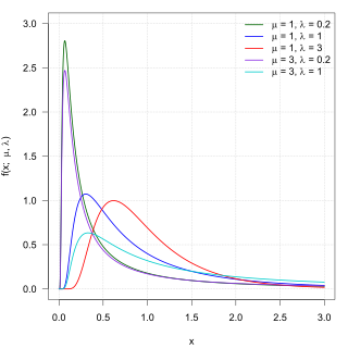
In probability theory, the inverse Gaussian distribution is a two-parameter family of continuous probability distributions with support on (0,∞).
Expected shortfall (ES) is a risk measure—a concept used in the field of financial risk measurement to evaluate the market risk or credit risk of a portfolio. The "expected shortfall at q% level" is the expected return on the portfolio in the worst of cases. ES is an alternative to value at risk that is more sensitive to the shape of the tail of the loss distribution.
A ratio distribution is a probability distribution constructed as the distribution of the ratio of random variables having two other known distributions. Given two random variables X and Y, the distribution of the random variable Z that is formed as the ratio Z = X/Y is a ratio distribution.
In financial mathematics, tail value at risk (TVaR), also known as tail conditional expectation (TCE) or conditional tail expectation (CTE), is a risk measure associated with the more general value at risk. It quantifies the expected value of the loss given that an event outside a given probability level has occurred.
In mathematics, the spectral theory of ordinary differential equations is the part of spectral theory concerned with the determination of the spectrum and eigenfunction expansion associated with a linear ordinary differential equation. In his dissertation, Hermann Weyl generalized the classical Sturm–Liouville theory on a finite closed interval to second order differential operators with singularities at the endpoints of the interval, possibly semi-infinite or infinite. Unlike the classical case, the spectrum may no longer consist of just a countable set of eigenvalues, but may also contain a continuous part. In this case the eigenfunction expansion involves an integral over the continuous part with respect to a spectral measure, given by the Titchmarsh–Kodaira formula. The theory was put in its final simplified form for singular differential equations of even degree by Kodaira and others, using von Neumann's spectral theorem. It has had important applications in quantum mechanics, operator theory and harmonic analysis on semisimple Lie groups.

In probability theory and statistics, the normal-inverse-gamma distribution is a four-parameter family of multivariate continuous probability distributions. It is the conjugate prior of a normal distribution with unknown mean and variance.

In probability theory and statistics, the Poisson distribution is a discrete probability distribution that expresses the probability of a given number of events occurring in a fixed interval of time if these events occur with a known constant mean rate and independently of the time since the last event. It can also be used for the number of events in other types of intervals than time, and in dimension greater than 1.


