Applications and mapping algorithms
Both the true Hilbert curve and its discrete approximations are useful because they give a mapping between 1D and 2D space that preserves locality fairly well. [4] This means that two data points which are close to each other in one-dimensional space are also close to each other after folding. The converse cannot always be true.
Because of this locality property, the Hilbert curve is widely used in computer science. For example, the range of IP addresses used by computers can be mapped into a picture using the Hilbert curve. Code to generate the image would map from 2D to 1D to find the color of each pixel, and the Hilbert curve is sometimes used because it keeps nearby IP addresses close to each other in the picture. [5] The locality property of the Hilbert curve has also been used to design algorithms for exploring regions with mobile robots. [6] [7]
In an algorithm called Riemersma dithering, grayscale photographs can be converted to a dithered black-and-white image using thresholding, with the leftover amount from each pixel added to the next pixel along the Hilbert curve. Code to do this would map from 1D to 2D, and the Hilbert curve is sometimes used because it does not create the distracting patterns that would be visible to the eye if the order were simply left to right across each row of pixels. [8] Hilbert curves in higher dimensions are an instance of a generalization of Gray codes, and are sometimes used for similar purposes, for similar reasons. For multidimensional databases, Hilbert order has been proposed to be used instead of Z order because it has better locality-preserving behavior. For example, Hilbert curves have been used to compress and accelerate R-tree indexes [9] (see Hilbert R-tree). They have also been used to help compress data warehouses. [10] [11]
The linear distance of any point along the curve can be converted to coordinates in n dimensions for a given n, and vice versa, using any of several standard mathematical techniques such as Skilling's method. [12] [13]
It is possible to implement Hilbert curves efficiently even when the data space does not form a square. [14] Moreover, there are several possible generalizations of Hilbert curves to higher dimensions. [15] [16]

In mathematics, a fractal is a geometric shape containing detailed structure at arbitrarily small scales, usually having a fractal dimension strictly exceeding the topological dimension. Many fractals appear similar at various scales, as illustrated in successive magnifications of the Mandelbrot set. This exhibition of similar patterns at increasingly smaller scales is called self-similarity, also known as expanding symmetry or unfolding symmetry; if this replication is exactly the same at every scale, as in the Menger sponge, the shape is called affine self-similar. Fractal geometry lies within the mathematical branch of measure theory.

In mathematics, Hausdorff dimension is a measure of roughness, or more specifically, fractal dimension, that was introduced in 1918 by mathematician Felix Hausdorff. For instance, the Hausdorff dimension of a single point is zero, of a line segment is 1, of a square is 2, and of a cube is 3. That is, for sets of points that define a smooth shape or a shape that has a small number of corners—the shapes of traditional geometry and science—the Hausdorff dimension is an integer agreeing with the usual sense of dimension, also known as the topological dimension. However, formulas have also been developed that allow calculation of the dimension of other less simple objects, where, solely on the basis of their properties of scaling and self-similarity, one is led to the conclusion that particular objects—including fractals—have non-integer Hausdorff dimensions. Because of the significant technical advances made by Abram Samoilovitch Besicovitch allowing computation of dimensions for highly irregular or "rough" sets, this dimension is also commonly referred to as the Hausdorff–Besicovitch dimension.

The Mandelbrot set is a two-dimensional set with a relatively simple definition that exhibits great complexity, especially as it is magnified. It is popular for its aesthetic appeal and fractal structures. The set is defined in the complex plane as the complex numbers for which the function does not diverge to infinity when iterated starting at , i.e., for which the sequence , , etc., remains bounded in absolute value.
The Koch snowflake is a fractal curve and one of the earliest fractals to have been described. It is based on the Koch curve, which appeared in a 1904 paper titled "On a Continuous Curve Without Tangents, Constructible from Elementary Geometry" by the Swedish mathematician Helge von Koch.
In mathematics, a fractal dimension is a term invoked in the science of geometry to provide a rational statistical index of complexity detail in a pattern. A fractal pattern changes with the scale at which it is measured. It is also a measure of the space-filling capacity of a pattern, and it tells how a fractal scales differently, in a fractal (non-integer) dimension.
In mathematical analysis, a space-filling curve is a curve whose range reaches every point in a higher dimensional region, typically the unit square. Because Giuseppe Peano (1858–1932) was the first to discover one, space-filling curves in the 2-dimensional plane are sometimes called Peano curves, but that phrase also refers to the Peano curve, the specific example of a space-filling curve found by Peano.

In mathematics, when a mathematical phenomenon runs counter to some intuition, then the phenomenon is sometimes called pathological. On the other hand, if a phenomenon does not run counter to intuition, it is sometimes called well-behaved. These terms are sometimes useful in mathematical research and teaching, but there is no strict mathematical definition of pathological or well-behaved.
In mathematics, Hausdorff measure is a generalization of the traditional notions of area and volume to non-integer dimensions, specifically fractals and their Hausdorff dimensions. It is a type of outer measure, named for Felix Hausdorff, that assigns a number in [0,∞] to each set in or, more generally, in any metric space.

A quadtree is a tree data structure in which each internal node has exactly four children. Quadtrees are the two-dimensional analog of octrees and are most often used to partition a two-dimensional space by recursively subdividing it into four quadrants or regions. The data associated with a leaf cell varies by application, but the leaf cell represents a "unit of interesting spatial information".

In fractal geometry, the Minkowski–Bouligand dimension, also known as Minkowski dimension or box-counting dimension, is a way of determining the fractal dimension of a set in a Euclidean space , or more generally in a metric space . It is named after the Polish mathematician Hermann Minkowski and the French mathematician Georges Bouligand.
Sierpiński curves are a recursively defined sequence of continuous closed plane fractal curves discovered by Wacław Sierpiński, which in the limit completely fill the unit square: thus their limit curve, also called the Sierpiński curve, is an example of a space-filling curve.

In mathematical analysis and computer science, functions which are Z-order, Lebesgue curve, Morton space-filling curve, Morton order or Morton code map multidimensional data to one dimension while preserving locality of the data points. It is named in France after Henri Lebesgue, who studied it in 1904, and named in the United States after Guy Macdonald Morton, who first applied the order to file sequencing in 1966. The z-value of a point in multidimensions is simply calculated by interleaving the binary representations of its coordinate values. Once the data are sorted into this ordering, any one-dimensional data structure can be used, such as simple one dimensional arrays, binary search trees, B-trees, skip lists or hash tables. The resulting ordering can equivalently be described as the order one would get from a depth-first traversal of a quadtree or octree.

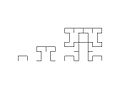
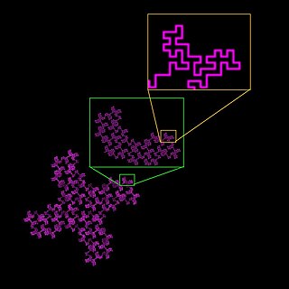
The Gosper curve, named after Bill Gosper, also known as the Peano-Gosper Curve and the flowsnake, is a space-filling curve whose limit set is rep-7. It is a fractal curve similar in its construction to the dragon curve and the Hilbert curve.
In fractal geometry, the H tree is a fractal tree structure constructed from perpendicular line segments, each smaller by a factor of the square root of 2 from the next larger adjacent segment. It is so called because its repeating pattern resembles the letter "H". It has Hausdorff dimension 2, and comes arbitrarily close to every point in a rectangle. Its applications include VLSI design and microwave engineering.
Hilbert R-tree, an R-tree variant, is an index for multidimensional objects such as lines, regions, 3-D objects, or high-dimensional feature-based parametric objects. It can be thought of as an extension to B+-tree for multidimensional objects.

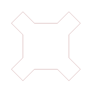
A Moore curve is a continuous fractal space-filling curve which is a variant of the Hilbert curve. Precisely, it is the loop version of the Hilbert curve, and it may be thought as the union of four copies of the Hilbert curves combined in such a way to make the endpoints coincide.
In computer science, the Bx tree is a query that is used to update efficient B+ tree-based index structures for moving objects.
Space-filling trees are geometric constructions that are analogous to space-filling curves, but have a branching, tree-like structure and are rooted. A space-filling tree is defined by an incremental process that results in a tree for which every point in the space has a finite-length path that converges to it. In contrast to space-filling curves, individual paths in the tree are short, allowing any part of the space to be quickly reached from the root. The simplest examples of space-filling trees have a regular, self-similar, fractal structure, but can be generalized to non-regular and even randomized/Monte-Carlo variants. Space-filling trees have interesting parallels in nature, including fluid distribution systems, vascular networks, and fractal plant growth, and many interesting connections to L-systems in computer science.
An n-flake, polyflake, or Sierpinski n-gon, is a fractal constructed starting from an n-gon. This n-gon is replaced by a flake of smaller n-gons, such that the scaled polygons are placed at the vertices, and sometimes in the center. This process is repeated recursively to result in the fractal. Typically, there is also the restriction that the n-gons must touch yet not overlap.
Box counting is a method of gathering data for analyzing complex patterns by breaking a dataset, object, image, etc. into smaller and smaller pieces, typically "box"-shaped, and analyzing the pieces at each smaller scale. The essence of the process has been compared to zooming in or out using optical or computer based methods to examine how observations of detail change with scale. In box counting, however, rather than changing the magnification or resolution of a lens, the investigator changes the size of the element used to inspect the object or pattern. Computer based box counting algorithms have been applied to patterns in 1-, 2-, and 3-dimensional spaces. The technique is usually implemented in software for use on patterns extracted from digital media, although the fundamental method can be used to investigate some patterns physically. The technique arose out of and is used in fractal analysis. It also has application in related fields such as lacunarity and multifractal analysis.