Applications include distributional clustering and dimension reduction, and more recently it has been suggested as a theoretical foundation for deep learning. It generalized the classical notion of minimal sufficient statistics from parametric statistics to arbitrary distributions, not necessarily of exponential form. It does so by relaxing the sufficiency condition to capture some fraction of the mutual information with the relevant variable Y.
The information bottleneck can also be viewed as a rate distortion problem, with a distortion function that measures how well Y is predicted from a compressed representation T compared to its direct prediction from X. This interpretation provides a general iterative algorithm for solving the information bottleneck trade-off and calculating the information curve from the distribution p(X,Y).
Let the compressed representation be given by random variable . The algorithm minimizes the following functional with respect to conditional distribution :
where and are the mutual information of and , and of and , respectively, and is a Lagrange multiplier.
Learning theory for deep learning
It has been mathematically proven that controlling information bottleneck is one way to control generalization error in deep learning.[2] Namely, the generalization error is proven to scale as where is the number of training samples, is the input to a deep neural network, and is the output of a hidden layer. This generalization bound scale with the degree of information bottleneck, unlike the other generalization bounds that scale with the number of parameters, VC dimension, Rademacher complexity, stability or robustness.
Phase transitions
This section is empty. You can help by adding to it. (December 2018)
Information theory of deep learning
Theory of Information Bottleneck is recently used to study Deep Neural Networks (DNN).[3] Consider and respectively as the input and output layers of a DNN, and let be any hidden layer of the network. Shwartz-Ziv and Tishby proposed the information bottleneck that expresses the tradeoff between the mutual information measures and . In this case, and respectively quantify the amount of information that the hidden layer contains about the input and the output. They conjectured that the training process of a DNN consists of two separate phases; 1) an initial fitting phase in which increases, and 2) a subsequent compression phase in which decreases. Saxe et al. in [4] countered the claim of Shwartz-Ziv and Tishby,[3] stating that this compression phenomenon in DNNs is not comprehensive, and it depends on the particular activation function. In particular, they claimed that the compression does not happen with ReLu activation functions. Shwartz-Ziv and Tishby disputed these claims, arguing that Saxe et al. had not observed compression due to weak estimates of the mutual information. Recently, Noshad et al. used a rate-optimal estimator of mutual information to explore this controversy, observing that the optimal hash-based estimator reveals the compression phenomenon in a wider range of networks with ReLu and maxpooling activations.[5] On the other hand, recently Goldfeld et al. have argued that the observed compression is a result of geometric, and not of information-theoretic phenomena,[6] a view that has been shared also in.[7]
Variational bottleneck
This section is empty. You can help by adding to it. (December 2018)
Gaussian bottleneck
The Gaussian bottleneck,[8] namely, applying the information bottleneck approach to Gaussian variables, leads to solutions related to canonical correlation analysis. Assume are jointly multivariate zero mean normal vectors with covariances and is a compressed version of that must maintain a given value of mutual information with . It can be shown that the optimum is a normal vector consisting of linear combinations of the elements of where matrix has orthogonal rows.
The projection matrix in fact contains rows selected from the weighted left eigenvectors of the singular value decomposition of the matrix (generally asymmetric)
Define the singular value decomposition
and the critical values
then the number of active eigenvectors in the projection, or order of approximation, is given by
And we finally get
In which the weights are given by
where
Applying the Gaussian information bottleneck to time series (processes), yields solutions related to optimal predictive coding. This procedure is formally equivalent to linear Slow Feature Analysis.[9]
Optimal temporal structures in linear dynamic systems can be revealed in the so-called past-future information bottleneck, an application of the bottleneck method to non-Gaussian sampled data.[10] The concept, as treated by Creutzig, Tishby et al., is not without complication as two independent phases make up in the exercise: firstly estimation of the unknown parent probability densities from which the data samples are drawn and secondly the use of these densities within the information theoretic framework of the bottleneck.
Since the bottleneck method is framed in probabilistic rather than statistical terms, the underlying probability density at the sample points must be estimated. This is a well known problem with multiple solutions described by Silverman.[11] In the present method, joint sample probabilities are found by use of a Markov transition matrix method and this has some mathematical synergy with the bottleneck method itself.
The arbitrarily increasing distance metric between all sample pairs and distance matrix is . Then transition probabilities between sample pairs for some must be computed. Treating samples as states, and a normalised version of as a Markov state transition probability matrix, the vector of probabilities of the 'states' after steps, conditioned on the initial state , is . The equilibrium probability vector given, in the usual way, by the dominant eigenvector of matrix which is independent of the initialising vector . This Markov transition method establishes a probability at the sample points which is claimed to be proportional to the probabilities' densities there.
Other interpretations of the use of the eigenvalues of distance matrix are discussed in Silverman's Density Estimation for Statistics and Data Analysis.[11]
Clusters
In the following soft clustering example, the reference vector contains sample categories and the joint probability is assumed known. A soft cluster is defined by its probability distribution over the data samples . Tishby et al. presented[1] the following iterative set of equations to determine the clusters which are ultimately a generalization of the Blahut-Arimoto algorithm, developed in rate distortion theory. The application of this type of algorithm in neural networks appears to originate in entropy arguments arising in the application of Gibbs Distributions in deterministic annealing.[12][13]
The function of each line of the iteration expands as
Line 1: This is a matrix valued set of conditional probabilities
The Kullback–Leibler divergence between the vectors generated by the sample data and those generated by its reduced information proxy is applied to assess the fidelity of the compressed vector with respect to the reference (or categorical) data in accordance with the fundamental bottleneck equation. is the Kullback–Leibler divergence between distributions
and is a scalar normalization. The weighting by the negative exponent of the distance means that prior cluster probabilities are downweighted in line 1 when the Kullback–Leibler divergence is large, thus successful clusters grow in probability while unsuccessful ones decay.
Line 2: Second matrix-valued set of conditional probabilities. By definition
where the Bayes identities are used.
Line 3: this line finds the marginal distribution of the clusters
This is a standard result.
Further inputs to the algorithm are the marginal sample distribution which has already been determined by the dominant eigenvector of and the matrix valued Kullback–Leibler divergence function
derived from the sample spacings and transition probabilities.
The matrix can be initialized randomly or with a reasonable guess, while matrix needs no prior values. Although the algorithm converges, multiple minima may exist that would need to be resolved.[14]
Defining decision contours
To categorize a new sample external to the training set , the previous distance metric finds the transition probabilities between and all samples in , with a normalization. Secondly apply the last two lines of the 3-line algorithm to get cluster and conditional category probabilities.
Finally
Parameter must be kept under close supervision since, as it is increased from zero, increasing numbers of features, in the category probability space, snap into focus at certain critical thresholds.
An example
The following case examines clustering in a four quadrant multiplier with random inputs and two categories of output, , generated by . This function has two spatially separated clusters for each category and so demonstrates that the method can handle such distributions.
20 samples are taken, uniformly distributed on the square . The number of clusters used beyond the number of categories, two in this case, has little effect on performance and the results are shown for two clusters using parameters .
The distance function is where while the conditional distribution is a 2×20 matrix
and zero elsewhere.
The summation in line 2 incorporates only two values representing the training values of +1 or −1, but nevertheless works well. The figure shows the locations of the twenty samples with '0' representing Y = 1 and 'x' representing Y = −1. The contour at the unity likelihood ratio level is shown,
as a new sample is scanned over the square. Theoretically the contour should align with the and coordinates but for such small sample numbers they have instead followed the spurious clusterings of the sample points.
Decision contours
Neural network/fuzzy logic analogies
This algorithm is somewhat analogous to a neural network with a single hidden layer. The internal nodes are represented by the clusters and the first and second layers of network weights are the conditional probabilities and respectively. However, unlike a standard neural network, the algorithm relies entirely on probabilities as inputs rather than the sample values themselves, while internal and output values are all conditional probability density distributions. Nonlinear functions are encapsulated in distance metric (or influence functions/radial basis functions) and transition probabilities instead of sigmoid functions.
The Blahut-Arimoto three-line algorithm converges rapidly, often in tens of iterations, and by varying , and and the cardinality of the clusters, various levels of focus on features can be achieved.
The statistical soft clustering definition has some overlap with the verbal fuzzy membership concept of fuzzy logic.
Extensions
An interesting extension is the case of information bottleneck with side information.[15] Here information is maximized about one target variable and minimized about another, learning a representation that is informative about selected aspects of data. Formally
In probability theory and statistics, the exponential distribution or negative exponential distribution is the probability distribution of the distance between events in a Poisson point process, i.e., a process in which events occur continuously and independently at a constant average rate; the distance parameter could be any meaningful mono-dimensional measure of the process, such as time between production errors, or length along a roll of fabric in the weaving manufacturing process. It is a particular case of the gamma distribution. It is the continuous analogue of the geometric distribution, and it has the key property of being memoryless. In addition to being used for the analysis of Poisson point processes it is found in various other contexts.
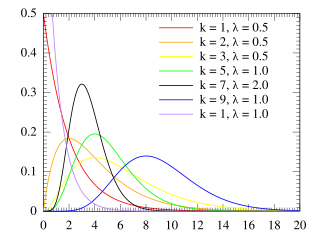
The Erlang distribution is a two-parameter family of continuous probability distributions with support . The two parameters are:
In probability theory and statistics, the Weibull distribution is a continuous probability distribution. It models a broad range of random variables, largely in the nature of a time to failure or time between events. Examples are maximum one-day rainfalls and the time a user spends on a web page.
The Ising model, named after the physicists Ernst Ising and Wilhelm Lenz, is a mathematical model of ferromagnetism in statistical mechanics. The model consists of discrete variables that represent magnetic dipole moments of atomic "spins" that can be in one of two states. The spins are arranged in a graph, usually a lattice, allowing each spin to interact with its neighbors. Neighboring spins that agree have a lower energy than those that disagree; the system tends to the lowest energy but heat disturbs this tendency, thus creating the possibility of different structural phases. The model allows the identification of phase transitions as a simplified model of reality. The two-dimensional square-lattice Ising model is one of the simplest statistical models to show a phase transition.
In physics, a partition function describes the statistical properties of a system in thermodynamic equilibrium. Partition functions are functions of the thermodynamic state variables, such as the temperature and volume. Most of the aggregate thermodynamic variables of the system, such as the total energy, free energy, entropy, and pressure, can be expressed in terms of the partition function or its derivatives. The partition function is dimensionless.
The Gell-Mann matrices, developed by Murray Gell-Mann, are a set of eight linearly independent 3×3 traceless Hermitian matrices used in the study of the strong interaction in particle physics. They span the Lie algebra of the SU(3) group in the defining representation.
A continuous-time Markov chain (CTMC) is a continuous stochastic process in which, for each state, the process will change state according to an exponential random variable and then move to a different state as specified by the probabilities of a stochastic matrix. An equivalent formulation describes the process as changing state according to the least value of a set of exponential random variables, one for each possible state it can move to, with the parameters determined by the current state.
In statistics, the theory of minimum norm quadratic unbiased estimation (MINQUE) was developed by C. R. Rao. MINQUE is a theory alongside other estimation methods in estimation theory, such as the method of moments or maximum likelihood estimation. Similar to the theory of best linear unbiased estimation, MINQUE is specifically concerned with linear regression models. The method was originally conceived to estimate heteroscedastic error variance in multiple linear regression. MINQUE estimators also provide an alternative to maximum likelihood estimators or restricted maximum likelihood estimators for variance components in mixed effects models. MINQUE estimators are quadratic forms of the response variable and are used to estimate a linear function of the variances.
In probability theory and mathematical physics, a random matrix is a matrix-valued random variable—that is, a matrix in which some or all elements are random variables. Many important properties of physical systems can be represented mathematically as matrix problems. For example, the thermal conductivity of a lattice can be computed from the dynamical matrix of the particle-particle interactions within the lattice.
The Lanczos algorithm is an iterative method devised by Cornelius Lanczos that is an adaptation of power methods to find the "most useful" eigenvalues and eigenvectors of an Hermitian matrix, where is often but not necessarily much smaller than . Although computationally efficient in principle, the method as initially formulated was not useful, due to its numerical instability.
A phase-type distribution is a probability distribution constructed by a convolution or mixture of exponential distributions. It results from a system of one or more inter-related Poisson processes occurring in sequence, or phases. The sequence in which each of the phases occurs may itself be a stochastic process. The distribution can be represented by a random variable describing the time until absorption of a Markov process with one absorbing state. Each of the states of the Markov process represents one of the phases.
Proportional hazards models are a class of survival models in statistics. Survival models relate the time that passes, before some event occurs, to one or more covariates that may be associated with that quantity of time. In a proportional hazards model, the unique effect of a unit increase in a covariate is multiplicative with respect to the hazard rate. For example, taking a drug may halve one's hazard rate for a stroke occurring, or, changing the material from which a manufactured component is constructed may double its hazard rate for failure. Other types of survival models such as accelerated failure time models do not exhibit proportional hazards. The accelerated failure time model describes a situation where the biological or mechanical life history of an event is accelerated.
In probability theory, Dirichlet processes are a family of stochastic processes whose realizations are probability distributions. In other words, a Dirichlet process is a probability distribution whose range is itself a set of probability distributions. It is often used in Bayesian inference to describe the prior knowledge about the distribution of random variables—how likely it is that the random variables are distributed according to one or another particular distribution.
A ratio distribution is a probability distribution constructed as the distribution of the ratio of random variables having two other known distributions. Given two random variables X and Y, the distribution of the random variable Z that is formed as the ratio Z = X/Y is a ratio distribution.
In the field of mathematical modeling, a radial basis function network is an artificial neural network that uses radial basis functions as activation functions. The output of the network is a linear combination of radial basis functions of the inputs and neuron parameters. Radial basis function networks have many uses, including function approximation, time series prediction, classification, and system control. They were first formulated in a 1988 paper by Broomhead and Lowe, both researchers at the Royal Signals and Radar Establishment.
In statistics and machine learning, lasso is a regression analysis method that performs both variable selection and regularization in order to enhance the prediction accuracy and interpretability of the resulting statistical model. The lasso method assumes that the coefficients of the linear model are sparse, meaning that few of them are non-zero. It was originally introduced in geophysics, and later by Robert Tibshirani, who coined the term.
In probability theory and statistics, the Poisson distribution is a discrete probability distribution that expresses the probability of a given number of events occurring in a fixed interval of time if these events occur with a known constant mean rate and independently of the time since the last event. It can also be used for the number of events in other types of intervals than time, and in dimension greater than 1.
The multivariate stable distribution is a multivariate probability distribution that is a multivariate generalisation of the univariate stable distribution. The multivariate stable distribution defines linear relations between stable distribution marginals. In the same way as for the univariate case, the distribution is defined in terms of its characteristic function.
In machine learning, the kernel embedding of distributions comprises a class of nonparametric methods in which a probability distribution is represented as an element of a reproducing kernel Hilbert space (RKHS). A generalization of the individual data-point feature mapping done in classical kernel methods, the embedding of distributions into infinite-dimensional feature spaces can preserve all of the statistical features of arbitrary distributions, while allowing one to compare and manipulate distributions using Hilbert space operations such as inner products, distances, projections, linear transformations, and spectral analysis. This learning framework is very general and can be applied to distributions over any space on which a sensible kernel function may be defined. For example, various kernels have been proposed for learning from data which are: vectors in , discrete classes/categories, strings, graphs/networks, images, time series, manifolds, dynamical systems, and other structured objects. The theory behind kernel embeddings of distributions has been primarily developed by Alex Smola, Le Song , Arthur Gretton, and Bernhard Schölkopf. A review of recent works on kernel embedding of distributions can be found in.
Tau functions are an important ingredient in the modern mathematical theory of integrable systems, and have numerous applications in a variety of other domains. They were originally introduced by Ryogo Hirota in his direct method approach to soliton equations, based on expressing them in an equivalent bilinear form.
↑ Slonim, Noam; Tishby, Naftali (2000-01-01). "Document clustering using word clusters via the information bottleneck method". Proceedings of the 23rd annual international ACM SIGIR conference on Research and development in information retrieval. SIGIR '00. New York, NY, USA: ACM. pp.208–215. CiteSeerX10.1.1.21.3062. doi:10.1145/345508.345578. ISBN978-1-58113-226-7. S2CID1373541.
↑ D. J. Miller, A. V. Rao, K. Rose, A. Gersho: "An Information-theoretic Learning Algorithm for Neural Network Classification". NIPS 1995: pp.591–597
This page is based on this Wikipedia article Text is available under the CC BY-SA 4.0 license; additional terms may apply. Images, videos and audio are available under their respective licenses.