Intrinsic dimension

Last updated

The intrinsic dimension for a data set can be thought of as the number of variables needed in a minimal representation of the data. Similarly, in signal processing of multidimensional signals, the intrinsic dimension of the signal describes how many variables are needed to generate a good approximation of the signal.

Contents

When estimating intrinsic dimension, however, a slightly broader definition based on manifold dimension is often used, where a representation in the intrinsic dimension does only need to exist locally. Such intrinsic dimension estimation methods can thus handle data sets with different intrinsic dimensions in different parts of the data set. This is often referred to as local intrinsic dimensionality.

The intrinsic dimension can be used as a lower bound of what dimension it is possible to compress a data set into through dimension reduction, but it can also be used as a measure of the complexity of the data set or signal. For a data set or signal of N variables, its intrinsic dimension M satisfies 0 M N, although estimators may yield higher values.

Example

Let be a two-variable function (or signal) which is of the form for some one-variable function g which is not constant. This means that f varies, in accordance to g, with the first variable or along the first coordinate. On the other hand, f is constant with respect to the second variable or along the second coordinate. It is only necessary to know the value of one, namely the first, variable in order to determine the value of f. Hence, it is a two-variable function but its intrinsic dimension is one.

A slightly more complicated example is. f is still intrinsic one-dimensional, which can be seen by making a variable transformation and which gives . Since the variation in f can be described by the single variable y1 its intrinsic dimension is one.

For the case that f is constant, its intrinsic dimension is zero since no variable is needed to describe variation. For the general case, when the intrinsic dimension of the two-variable function f is neither zero or one, it is two.

In the literature, functions which are of intrinsic dimension zero, one, or two are sometimes referred to as i0D, i1D or i2D, respectively.

Formal definition for signals

For an N-variable function f, the set of variables can be represented as an N-dimensional vector x: .

If for some M-variable function g and M × N matrix A is it the case that

then the intrinsic dimension of f is M.

The intrinsic dimension is a characterization of f, it is not an unambiguous characterization of g nor of A. That is, if the above relation is satisfied for some f, g, and A, it must also be satisfied for the same f and g and A given by and where B is a non-singular M × M matrix, since .

The Fourier transform of signals of low intrinsic dimension

An N variable function which has intrinsic dimension M < N has a characteristic Fourier transform. Intuitively, since this type of function is constant along one or several dimensions its Fourier transform must appear like an impulse (the Fourier transform of a constant) along the same dimension in the frequency domain.

A simple example

Let f be a two-variable function which is i1D. This means that there exists a normalized vector and a one-variable function g such that for all . If F is the Fourier transform of f (both are two-variable functions) it must be the case that .

Here G is the Fourier transform of g (both are one-variable functions), δ is the Dirac impulse function and m is a normalized vector in perpendicular to n. This means that F vanishes everywhere except on a line which passes through the origin of the frequency domain and is parallel to m. Along this line F varies according to G.

The general case

Let f be an N-variable function which has intrinsic dimension M, that is, there exists an M-variable function g and M × N matrix A such that .

Its Fourier transform F can then be described as follows:

Generalizations

The type of intrinsic dimension described above assumes that a linear transformation is applied to the coordinates of the N-variable function f to produce the M variables which are necessary to represent every value of f. This means that f is constant along lines, planes, or hyperplanes, depending on N and M.

In a general case, f has intrinsic dimension M if there exist M functions a1, a2, ..., aM and an M-variable function g such that

A simple example is transforming a 2-variable function f to polar coordinates:

For the general case, a simple description of either the point sets for which f is constant or its Fourier transform is usually not possible.

Local Intrinsic Dimensionality

Local intrinsic dimensionality (LID) refers to the observation that often data is distributed on a lower-dimensional manifold when only considering a nearby subset of the data. For example the function can be considered one-dimensional when y is close to 0 (with one variable x), two-dimensional when y is close to 1, and again one-dimensional when y is positive and much larger than 1 (with variable x+y).

Local intrinsic dimensionality is often used with respect to data. It then usually is estimated based on the k nearest neighbors of a data point, [1] often based on a concept related to the doubling dimension in mathematics. Since the volume of a d-sphere grows exponentially in d, the rate at which new neighbors are found as the search radius is increased can be used to estimate the local intrinsic dimensionality (e.g., GED estimation [2] ). However, alternate approaches of estimation have been proposed, for example angle-based estimation. [3]

Intrinsic dimension estimation

Intrinsic dimension of data manifolds can be estimated by many methods, depending on assumptions of the data manifold. A 2016 review is. [4]

The two-nearest neighbors (TwoNN) method is a method for estimating the intrinsic dimension of an immersed Riemannian manifold. The algorithm is as follows: [5]

Scatter some points on the manifold.

Measure for many points, where are the distances to the point's two closest neighbors.

Fit the empirical CDF of to .

Return .

History

During the 1950s so called "scaling" methods were developed in the social sciences to explore and summarize multidimensional data sets. [6] After Shepard introduced non-metric multidimensional scaling in 1962 [7] one of the major research areas within multi-dimensional scaling (MDS) was estimation of the intrinsic dimension. [8] The topic was also studied in information theory, pioneered by Bennet in 1965 who coined the term "intrinsic dimension" and wrote a computer program to estimate it. [9] [10] [11]

During the 1970s intrinsic dimensionality estimation methods were constructed that did not depend on dimensionality reductions such as MDS: based on local eigenvalues., [12] based on distance distributions, [13] and based on other dimension-dependent geometric properties [14]

Estimating intrinsic dimension of sets and probability measures has also been extensively studied since around 1980 in the field of dynamical systems, where dimensions of (strange) attractors have been the subject of interest. [15] [16] [17] [18] For strange attractors there is no manifold assumption, and the dimension measured is some version of fractal dimension — which also can be non-integer. However, definitions of fractal dimension yield the manifold dimension for manifolds.

In the 2000s the "curse of dimensionality" has been exploited to estimate intrinsic dimension. [19] [20]

Applications

The case of a two-variable signal which is i1D appears frequently in computer vision and image processing and captures the idea of local image regions which contain lines or edges. The analysis of such regions has a long history, but it was not until a more formal and theoretical treatment of such operations began that the concept of intrinsic dimension was established, even though the name has varied.

For example, the concept which here is referred to as an image neighborhood of intrinsic dimension 1 or i1D neighborhood is called 1-dimensional by Knutsson (1982), [21] linear symmetric by Bigün & Granlund (1987) [22] and simple neighborhood in Granlund & Knutsson (1995). [23]

See also

Related Research Articles

<span class="mw-page-title-main">Autocorrelation</span> Correlation of a signal with a time-shifted copy of itself, as a function of shift

Autocorrelation, sometimes known as serial correlation in the discrete time case, is the correlation of a signal with a delayed copy of itself as a function of delay. Informally, it is the similarity between observations of a random variable as a function of the time lag between them. The analysis of autocorrelation is a mathematical tool for finding repeating patterns, such as the presence of a periodic signal obscured by noise, or identifying the missing fundamental frequency in a signal implied by its harmonic frequencies. It is often used in signal processing for analyzing functions or series of values, such as time domain signals.

<span class="mw-page-title-main">Convolution</span> Integral expressing the amount of overlap of one function as it is shifted over another

In mathematics, convolution is a mathematical operation on two functions that produces a third function. The term convolution refers to both the result function and to the process of computing it. It is defined as the integral of the product of the two functions after one is reflected about the y-axis and shifted. The integral is evaluated for all values of shift, producing the convolution function. The choice of which function is reflected and shifted before the integral does not change the integral result. Graphically, it expresses how the 'shape' of one function is modified by the other.

<span class="mw-page-title-main">Discrete Fourier transform</span> Type of Fourier transform in discrete mathematics

In mathematics, the discrete Fourier transform (DFT) converts a finite sequence of equally-spaced samples of a function into a same-length sequence of equally-spaced samples of the discrete-time Fourier transform (DTFT), which is a complex-valued function of frequency. The interval at which the DTFT is sampled is the reciprocal of the duration of the input sequence. An inverse DFT (IDFT) is a Fourier series, using the DTFT samples as coefficients of complex sinusoids at the corresponding DTFT frequencies. It has the same sample-values as the original input sequence. The DFT is therefore said to be a frequency domain representation of the original input sequence. If the original sequence spans all the non-zero values of a function, its DTFT is continuous, and the DFT provides discrete samples of one cycle. If the original sequence is one cycle of a periodic function, the DFT provides all the non-zero values of one DTFT cycle.

In mathematics, and more specifically in linear algebra, a linear map is a mapping between two vector spaces that preserves the operations of vector addition and scalar multiplication. The same names and the same definition are also used for the more general case of modules over a ring; see Module homomorphism.

<span class="mw-page-title-main">Dirac delta function</span> Generalized function whose value is zero everywhere except at zero

In mathematical analysis, the Dirac delta function, also known as the unit impulse, is a generalized function on the real numbers, whose value is zero everywhere except at zero, and whose integral over the entire real line is equal to one. Since there is no function having this property, to model the delta "function" rigorously involves the use of limits or, as is common in mathematics, measure theory and the theory of distributions.

<span class="mw-page-title-main">Fourier transform</span> Mathematical transform that expresses a function of time as a function of frequency

In physics, engineering and mathematics, the Fourier transform (FT) is an integral transform that converts a function into a form that describes the frequencies present in the original function. The output of the transform is a complex-valued function of frequency. The term Fourier transform refers to both this complex-valued function and the mathematical operation. When a distinction needs to be made the Fourier transform is sometimes called the frequency domain representation of the original function. The Fourier transform is analogous to decomposing the sound of a musical chord into the intensities of its constituent pitches.

<span class="mw-page-title-main">Fourier series</span> Decomposition of periodic functions into sums of simpler sinusoidal forms

A Fourier series is an expansion of a periodic function into a sum of trigonometric functions. The Fourier series is an example of a trigonometric series, but not all trigonometric series are Fourier series. By expressing a function as a sum of sines and cosines, many problems involving the function become easier to analyze because trigonometric functions are well understood. For example, Fourier series were first used by Joseph Fourier to find solutions to the heat equation. This application is possible because the derivatives of trigonometric functions fall into simple patterns. Fourier series cannot be used to approximate arbitrary functions, because most functions have infinitely many terms in their Fourier series, and the series do not always converge. Well-behaved functions, for example smooth functions, have Fourier series that converge to the original function. The coefficients of the Fourier series are determined by integrals of the function multiplied by trigonometric functions, described in Common forms of the Fourier series below.

In mathematics, a Gaussian function, often simply referred to as a Gaussian, is a function of the base form

<span class="mw-page-title-main">Legendre transformation</span> Mathematical transformation

In mathematics, the Legendre transformation, first introduced by Adrien-Marie Legendre in 1787 when studying the minimal surface problem, is an involutive transformation on real-valued functions that are convex on a real variable. Specifically, if a real-valued multivariable function is convex on one of its independent real variables, then the Legendre transform with respect to this variable is applicable to the function.

<span class="mw-page-title-main">Radon transform</span> Integral transform

In mathematics, the Radon transform is the integral transform which takes a function f defined on the plane to a function Rf defined on the (two-dimensional) space of lines in the plane, whose value at a particular line is equal to the line integral of the function over that line. The transform was introduced in 1917 by Johann Radon, who also provided a formula for the inverse transform. Radon further included formulas for the transform in three dimensions, in which the integral is taken over planes. It was later generalized to higher-dimensional Euclidean spaces and more broadly in the context of integral geometry. The complex analogue of the Radon transform is known as the Penrose transform. The Radon transform is widely applicable to tomography, the creation of an image from the projection data associated with cross-sectional scans of an object.

<span class="mw-page-title-main">Reciprocal lattice</span> Fourier transform of a real-space lattice, important in solid-state physics

In physics, the reciprocal lattice emerges from the Fourier transform of another lattice. The direct lattice or real lattice is a periodic function in physical space, such as a crystal system. The reciprocal lattice exists in the mathematical space of spatial frequencies, known as reciprocal space or k space, where refers to the wavevector.

<span class="mw-page-title-main">Cross-correlation</span> Covariance and correlation

In signal processing, cross-correlation is a measure of similarity of two series as a function of the displacement of one relative to the other. This is also known as a sliding dot product or sliding inner-product. It is commonly used for searching a long signal for a shorter, known feature. It has applications in pattern recognition, single particle analysis, electron tomography, averaging, cryptanalysis, and neurophysiology. The cross-correlation is similar in nature to the convolution of two functions. In an autocorrelation, which is the cross-correlation of a signal with itself, there will always be a peak at a lag of zero, and its size will be the signal energy.

In mathematics, the Helmholtz equation is the eigenvalue problem for the Laplace operator. It corresponds to the linear partial differential equation

<span class="mw-page-title-main">Array processing</span>

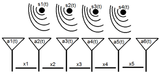
Array processing is a wide area of research in the field of signal processing that extends from the simplest form of 1 dimensional line arrays to 2 and 3 dimensional array geometries. Array structure can be defined as a set of sensors that are spatially separated, e.g. radio antenna and seismic arrays. The sensors used for a specific problem may vary widely, for example microphones, accelerometers and telescopes. However, many similarities exist, the most fundamental of which may be an assumption of wave propagation. Wave propagation means there is a systemic relationship between the signal received on spatially separated sensors. By creating a physical model of the wave propagation, or in machine learning applications a training data set, the relationships between the signals received on spatially separated sensors can be leveraged for many applications.

In mathematics, the discrete Laplace operator is an analog of the continuous Laplace operator, defined so that it has meaning on a graph or a discrete grid. For the case of a finite-dimensional graph, the discrete Laplace operator is more commonly called the Laplacian matrix.

In mathematics, the Hankel transform expresses any given function f(r) as the weighted sum of an infinite number of Bessel functions of the first kind Jν(kr). The Bessel functions in the sum are all of the same order ν, but differ in a scaling factor k along the r axis. The necessary coefficient Fν of each Bessel function in the sum, as a function of the scaling factor k constitutes the transformed function. The Hankel transform is an integral transform and was first developed by the mathematician Hermann Hankel. It is also known as the Fourier–Bessel transform. Just as the Fourier transform for an infinite interval is related to the Fourier series over a finite interval, so the Hankel transform over an infinite interval is related to the Fourier–Bessel series over a finite interval.

<span class="mw-page-title-main">Characteristic function (probability theory)</span> Fourier transform of the probability density function

In probability theory and statistics, the characteristic function of any real-valued random variable completely defines its probability distribution. If a random variable admits a probability density function, then the characteristic function is the Fourier transform of the probability density function. Thus it provides an alternative route to analytical results compared with working directly with probability density functions or cumulative distribution functions. There are particularly simple results for the characteristic functions of distributions defined by the weighted sums of random variables.

In directional statistics, the von Mises–Fisher distribution, is a probability distribution on the -sphere in . If the distribution reduces to the von Mises distribution on the circle.

Phase retrieval is the process of algorithmically finding solutions to the phase problem. Given a complex signal , of amplitude , and phase :

Kernel density estimation is a nonparametric technique for density estimation i.e., estimation of probability density functions, which is one of the fundamental questions in statistics. It can be viewed as a generalisation of histogram density estimation with improved statistical properties. Apart from histograms, other types of density estimators include parametric, spline, wavelet and Fourier series. Kernel density estimators were first introduced in the scientific literature for univariate data in the 1950s and 1960s and subsequently have been widely adopted. It was soon recognised that analogous estimators for multivariate data would be an important addition to multivariate statistics. Based on research carried out in the 1990s and 2000s, multivariate kernel density estimation has reached a level of maturity comparable to its univariate counterparts.

References

  1. Amsaleg, Laurent; Chelly, Oussama; Furon, Teddy; Girard, Stéphane; Houle, Michael E.; Kawarabayashi, Ken-ichi; Nett, Michael (2015-08-10). "Estimating Local Intrinsic Dimensionality". Proceedings of the 21th ACM SIGKDD International Conference on Knowledge Discovery and Data Mining. KDD '15. Sydney, NSW, Australia: Association for Computing Machinery. pp. 29–38. doi:10.1145/2783258.2783405. ISBN   978-1-4503-3664-2. S2CID   16058196.
  2. Houle, M. E.; Kashima, H.; Nett, M. (2012). "Generalized Expansion Dimension". 2012 IEEE 12th International Conference on Data Mining Workshops. pp. 587–594. doi:10.1109/ICDMW.2012.94. ISBN   978-1-4673-5164-5. S2CID   8336466.
  3. Thordsen, Erik; Schubert, Erich (2020). Satoh, Shin'ichi; Vadicamo, Lucia; Zimek, Arthur; Carrara, Fabio; Bartolini, Ilaria; Aumüller, Martin; Jónsson, Björn Þór; Pagh, Rasmus (eds.). "ABID: Angle Based Intrinsic Dimensionality". Similarity Search and Applications. Lecture Notes in Computer Science. Cham: Springer International Publishing. 12440: 218–232. arXiv: 2006.12880 . doi:10.1007/978-3-030-60936-8_17. ISBN   978-3-030-60936-8. S2CID   219980390.
  4. Camastra, Francesco; Staiano, Antonino (2016-01-20). "Intrinsic dimension estimation: Advances and open problems". Information Sciences. 328: 26–41. doi:10.1016/j.ins.2015.08.029. ISSN   0020-0255.
  5. Facco, Elena; d’Errico, Maria; Rodriguez, Alex; Laio, Alessandro (2017-09-22). "Estimating the intrinsic dimension of datasets by a minimal neighborhood information". Scientific Reports. 7 (1). arXiv: 1803.06992 . doi: 10.1038/s41598-017-11873-y . ISSN   2045-2322.
  6. Torgerson, Warren S. (1978) [1958]. Theory and methods of scaling. Wiley. ISBN   0471879452. OCLC   256008416.
  7. Shepard, Roger N. (1962). "The analysis of proximities: Multidimensional scaling with an unknown distance function. I.". Psychometrika. 27 (2): 125–140. doi:10.1007/BF02289630. S2CID   186222646.
  8. Shepard, Roger N. (1974). "Representation of structure in similarity data: Problems and prospects". Psychometrika. 39 (4): 373–421. doi:10.1007/BF02291665. S2CID   121704645.
  9. Bennet, Robert S. (June 1965). "Representation and analysis of signals—Part XXI: The intrinsic dimensionality of signal collections". Rep. 163. Baltimore, MD: The Johns Hopkins University.
  10. Robert S. Bennett (1965). Representation and Analysis of Signals Part XXI. The intrinsic dimensionality of signal collections (PDF) (PhD). Ann Arbor, Michigan: The Johns Hopkins University. Archived from the original (PDF) on December 27, 2019.
  11. Bennett, Robert S. (September 1969). "The intrinsic dimensionality of signal collections". IEEE Transactions on Information Theory. 15 (5): 517–525. doi:10.1109/TIT.1969.1054365.
  12. Fukunaga, K.; Olsen, D. R. (1971). "An algorithm for finding intrinsic dimensionality of data". IEEE Transactions on Computers. 20 (2): 176–183. doi:10.1109/T-C.1971.223208. S2CID   30206700.
  13. Pettis, K. W.; Bailey, Thomas A.; Jain, Anil K.; Dubes, Richard C. (1979). "An intrinsic dimensionality estimator from near-neighbor information". IEEE Transactions on Pattern Analysis and Machine Intelligence. 1 (1): 25–37. doi:10.1109/TPAMI.1979.4766873. PMID   21868828. S2CID   2196461.
  14. Trunk, G. V. (1976). "Statistical estimation of the intrinsic dimensionality of a noisy signal collection". IEEE Transactions on Computers. 100 (2): 165–171. doi:10.1109/TC.1976.5009231. S2CID   1181023.
  15. Grassberger, P.; Procaccia, I. (1983). "Measuring the strangeness of strange attractors". Physica D: Nonlinear Phenomena. 9 (1–2): 189–208. Bibcode:1983PhyD....9..189G. doi:10.1016/0167-2789(83)90298-1.
  16. Takens, F. (1984). "On the numerical determination of the dimension of an attractor". In Tong, Howell (ed.). Dynamical Systems and Bifurcations, Proceedings of a Workshop Held in Groningen, The Netherlands, April 16-20, 1984. Lecture Notes in Mathematics. Vol. 1125. Springer-Verlag. pp. 99–106. doi:10.1007/BFb0075637. ISBN   3540394117.
  17. Cutler, C. D. (1993). "A review of the theory and estimation of fractal dimension". Dimension estimation and models. Nonlinear Time Series and Chaos. Vol. 1. World Scientific. pp. 1–107. ISBN   9810213530.
  18. Harte, D. (2001). Multifractals — Theory and Applications. Chapman and Hall/CRC. ISBN   9781584881544.
  19. Chavez, E. (2001). "Searching in metric spaces". ACM Computing Surveys. 33 (3): 273–321. doi:10.1145/502807.502808. hdl: 10533/172863 . S2CID   3201604.
  20. Pestov, V. (2008). "An axiomatic approach to intrinsic dimension of a dataset". Neural Networks. 21 (2–3): 204–213. arXiv: 0712.2063 . doi:10.1016/j.neunet.2007.12.030. PMID   18234471. S2CID   2309396.
  21. Knutsson, Hans (1982). Filtering and reconstruction in image processing (PDF). Linköping Studies in Science and Technology. Vol. 88. Linköping University. ISBN   91-7372-595-1. oai:DiVA.org:liu-54890.
  22. Bigün, Josef; Granlund, Gösta H. (1987). "Optimal orientation detection of linear symmetry" (PDF). Proceedings of the International Conference on Computer Vision. pp. 433–438.
  23. Granlund, Gösta H.; Knutsson, Hans (1995). Signal Processing in Computer Vision. Kluwer Academic. ISBN   978-1-4757-2377-9.