Iterative deepening depth-first search

Last updated
Iterative deepening depth-first search
Class Search algorithm
Data structure Tree, Graph
Worst-case performance , where is the branching factor and is the depth of the shallowest solution
Worst-case space complexity [1] :5

In computer science, iterative deepening search or more specifically iterative deepening depth-first search [2] (IDS or IDDFS) is a state space/graph search strategy in which a depth-limited version of depth-first search is run repeatedly with increasing depth limits until the goal is found. IDDFS is optimal, meaning that it finds the shallowest goal. [3] Since it visits all the nodes in the search tree down to depth before visiting any nodes at depth , the cumulative order in which nodes are first visited is effectively the same as in breadth-first search. However, IDDFS uses much less memory. [1]

Contents

Algorithm for directed graphs

The following pseudocode shows IDDFS implemented in terms of a recursive depth-limited DFS (called DLS) for directed graphs. This implementation of IDDFS does not account for already-visited nodes.

function IDDFS(root) isfor depth from 0 todo         found, remaining ← DLS(root, depth)         if found ≠ nullthenreturn found         else if not remaining thenreturnnullfunction DLS(node, depth) isif depth = 0 thenif node is a goal thenreturn (node, true)         elsereturn (null, true)    (Not found, but may have children)else if depth > 0 then         any_remaining ← falseforeach child of node do             found, remaining ← DLS(child, depth−1)             if found ≠ null thenreturn (found, true)                if remaining then                 any_remaining ← true    (At least one node found at depth, let IDDFS deepen)return (null, any_remaining)

If the goal node is found by DLS, IDDFS will return it without looking deeper. Otherwise, if at least one node exists at that level of depth, the remaining flag will let IDDFS continue.

2-tuples are useful as return value to signal IDDFS to continue deepening or stop, in case tree depth and goal membership are unknown a priori. Another solution could use sentinel values instead to represent not found or remaining level results.

Properties

IDDFS achieves breadth-first search's completeness (when the branching factor is finite) using depth-first search's space-efficiency. If a solution exists, it will find a solution path with the fewest arcs. [3]

Iterative deepening visits states multiple times, and it may seem wasteful. However, if IDDFS explores a search tree to depth , most of the total effort is in exploring the states at depth . Relative to the number of states at depth , the cost of repeatedly visiting the states above this depth is always small. [4]

The main advantage of IDDFS in game tree searching is that the earlier searches tend to improve the commonly used heuristics, such as the killer heuristic and alpha–beta pruning, so that a more accurate estimate of the score of various nodes at the final depth search can occur, and the search completes more quickly since it is done in a better order. For example, alpha–beta pruning is most efficient if it searches the best moves first. [4]

A second advantage is the responsiveness of the algorithm. Because early iterations use small values for , they execute extremely quickly. This allows the algorithm to supply early indications of the result almost immediately, followed by refinements as increases. When used in an interactive setting, such as in a chess-playing program, this facility allows the program to play at any time with the current best move found in the search it has completed so far. This can be phrased as each depth of the search corecursively producing a better approximation of the solution, though the work done at each step is recursive. This is not possible with a traditional depth-first search, which does not produce intermediate results.

Asymptotic analysis

Time complexity

The time complexity of IDDFS in a (well-balanced) tree works out to be the same as breadth-first search, i.e. , [1] :5 where is the branching factor and is the depth of the goal.

Proof

In an iterative deepening search, the nodes at depth are expanded once, those at depth are expanded twice, and so on up to the root of the search tree, which is expanded times. [1] :5 So the total number of expansions in an iterative deepening search is

where is the number of expansions at depth , is the number of expansions at depth , and so on. Factoring out gives

Now let . Then we have

This is less than the infinite series

which converges to

, for

That is, we have

, for

Since or is a constant independent of (the depth), if (i.e., if the branching factor is greater than 1), the running time of the depth-first iterative deepening search is .

Example

For and the number is

All together, an iterative deepening search from depth all the way down to depth expands only about more nodes than a single breadth-first or depth-limited search to depth , when . [5]

The higher the branching factor, the lower the overhead of repeatedly expanded states, [1] :6 but even when the branching factor is 2, iterative deepening search only takes about twice as long as a complete breadth-first search. This means that the time complexity of iterative deepening is still .

Space complexity

The space complexity of IDDFS is , [1] :5 where is the depth of the goal.

Proof

Since IDDFS, at any point, is engaged in a depth-first search, it need only store a stack of nodes which represents the branch of the tree it is expanding. Since it finds a solution of optimal length, the maximum depth of this stack is , and hence the maximum amount of space is .

In general, iterative deepening is the preferred search method when there is a large search space and the depth of the solution is not known. [4]

Example

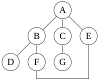
For the following graph:

Graph.traversal.example.svg

a depth-first search starting at A, assuming that the left edges in the shown graph are chosen before right edges, and assuming the search remembers previously-visited nodes and will not repeat them (since this is a small graph), will visit the nodes in the following order: A, B, D, F, E, C, G. The edges traversed in this search form a Trémaux tree, a structure with important applications in graph theory.

Performing the same search without remembering previously visited nodes results in visiting nodes in the order A, B, D, F, E, A, B, D, F, E, etc. forever, caught in the A, B, D, F, E cycle and never reaching C or G.

Iterative deepening prevents this loop and will reach the following nodes on the following depths, assuming it proceeds left-to-right as above:

(Iterative deepening has now seen C, when a conventional depth-first search did not.)

(It still sees C, but that it came later. Also it sees E via a different path, and loops back to F twice.)

For this graph, as more depth is added, the two cycles "ABFE" and "AEFB" will simply get longer before the algorithm gives up and tries another branch.

Similar to iterative deepening is a search strategy called iterative lengthening search that works with increasing path-cost limits instead of depth-limits. It expands nodes in the order of increasing path cost; therefore the first goal it encounters is the one with the cheapest path cost. But iterative lengthening incurs substantial overhead that makes it less useful than iterative deepening. [4]

Iterative deepening A* is a best-first search that performs iterative deepening based on "f"-values similar to the ones computed in the A* algorithm.

Bidirectional IDDFS

IDDFS has a bidirectional counterpart, [1] :6 which alternates two searches: one starting from the source node and moving along the directed arcs, and another one starting from the target node and proceeding along the directed arcs in opposite direction (from the arc's head node to the arc's tail node). The search process first checks that the source node and the target node are same, and if so, returns the trivial path consisting of a single source/target node. Otherwise, the forward search process expands the child nodes of the source node (set ), the backward search process expands the parent nodes of the target node (set ), and it is checked whether and intersect. If so, a shortest path is found. Otherwise, the search depth is incremented and the same computation takes place.

One limitation of the algorithm is that the shortest path consisting of an odd number of arcs will not be detected. Suppose we have a shortest path When the depth will reach two hops along the arcs, the forward search will proceed to from , and the backward search will proceed from to . Pictorially, the search frontiers will go through each other, and instead a suboptimal path consisting of an even number of arcs will be returned. This is illustrated in the below diagrams:

Bidirectional IDDFS Bidirectional iterative deepening depth-first search search frontier pass through each other.png
Bidirectional IDDFS

What comes to space complexity, the algorithm colors the deepest nodes in the forward search process in order to detect existence of the middle node where the two search processes meet.

Additional difficulty of applying bidirectional IDDFS is that if the source and the target nodes are in different strongly connected components, say, , if there is no arc leaving and entering , the search will never terminate.

Time and space complexities

The running time of bidirectional IDDFS is given by

and the space complexity is given by

where is the number of nodes in the shortest -path. Since the running time complexity of iterative deepening depth-first search is , the speedup is roughly

Pseudocode

function Build-Path(s, μ, B) isπ Find-Shortest-Path(s, μ) (Recursively compute the path to the relay node)     remove the last node from πreturnπ B (Append the backward search stack)
function Depth-Limited-Search-Forward(u, Δ, F) isifΔ = 0 then         F  F  {u} (Mark the node)returnforeach child of u do         Depth-Limited-Search-Forward(child, Δ − 1, F)
function Depth-Limited-Search-Backward(u, Δ, B, F) is     prepend u to B     ifΔ = 0 thenif u in F  thenreturn u (Reached the marked node, use it as a relay node)         remove the head node of B         return nullforeach parent of u doμ Depth-Limited-Search-Backward(parent, Δ − 1, B, F)         ifμnullthenreturnμ     remove the head node of B     return null
function Find-Shortest-Path(s, t) isif s = t thenreturn<s>    F, B, Δ, , 0    forever do        Depth-Limited-Search-Forward(s, Δ, F)        foreachδ = Δ, Δ + 1 doμ Depth-Limited-Search-Backward(t, δ, B, F)            ifμnull thenreturn Build-Path(s, μ, B) (Found a relay node)        F, Δ, Δ + 1

Related Research Articles

In number theory, an arithmetic, arithmetical, or number-theoretic function is for most authors any function f(n) whose domain is the positive integers and whose range is a subset of the complex numbers. Hardy & Wright include in their definition the requirement that an arithmetical function "expresses some arithmetical property of n".
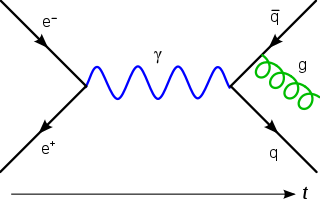
<span class="mw-page-title-main">Feynman diagram</span> Pictorial representation of the behavior of subatomic particles

In theoretical physics, a Feynman diagram is a pictorial representation of the mathematical expressions describing the behavior and interaction of subatomic particles. The scheme is named after American physicist Richard Feynman, who introduced the diagrams in 1948. The interaction of subatomic particles can be complex and difficult to understand; Feynman diagrams give a simple visualization of what would otherwise be an arcane and abstract formula. According to David Kaiser, "Since the middle of the 20th century, theoretical physicists have increasingly turned to this tool to help them undertake critical calculations. Feynman diagrams have revolutionized nearly every aspect of theoretical physics." While the diagrams are applied primarily to quantum field theory, they can also be used in other areas of physics, such as solid-state theory. Frank Wilczek wrote that the calculations that won him the 2004 Nobel Prize in Physics "would have been literally unthinkable without Feynman diagrams, as would [Wilczek's] calculations that established a route to production and observation of the Higgs particle."

In computer science, a red–black tree is a specialised binary search tree data structure noted for fast storage and retrieval of ordered information, and a guarantee that operations will complete within a known time. Compared to other self-balancing binary search trees, the nodes in a red-black tree hold an extra bit called "color" representing "red" and "black" which is used when re-organising the tree to ensure that it is always approximately balanced.
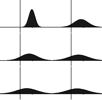
<span class="mw-page-title-main">Fokker–Planck equation</span> Partial differential equation

In statistical mechanics and information theory, the Fokker–Planck equation is a partial differential equation that describes the time evolution of the probability density function of the velocity of a particle under the influence of drag forces and random forces, as in Brownian motion. The equation can be generalized to other observables as well. The Fokker-Planck equation has multiple applications in information theory, graph theory, data science, finance, economics etc.

In mathematics, the Kronecker delta is a function of two variables, usually just non-negative integers. The function is 1 if the variables are equal, and 0 otherwise:

In the calculus of variations and classical mechanics, the Euler–Lagrange equations are a system of second-order ordinary differential equations whose solutions are stationary points of the given action functional. The equations were discovered in the 1750s by Swiss mathematician Leonhard Euler and Italian mathematician Joseph-Louis Lagrange.

In mathematics, the Hodge star operator or Hodge star is a linear map defined on the exterior algebra of a finite-dimensional oriented vector space endowed with a nondegenerate symmetric bilinear form. Applying the operator to an element of the algebra produces the Hodge dual of the element. This map was introduced by W. V. D. Hodge.

In bioinformatics, neighbor joining is a bottom-up (agglomerative) clustering method for the creation of phylogenetic trees, created by Naruya Saitou and Masatoshi Nei in 1987. Usually based on DNA or protein sequence data, the algorithm requires knowledge of the distance between each pair of taxa to create the phylogenetic tree.

<span class="mw-page-title-main">Path integral formulation</span> Formulation of quantum mechanics

The path integral formulation is a description in quantum mechanics that generalizes the action principle of classical mechanics. It replaces the classical notion of a single, unique classical trajectory for a system with a sum, or functional integral, over an infinity of quantum-mechanically possible trajectories to compute a quantum amplitude.

A directional derivative is a concept in multivariable calculus that measures the rate at which a function changes in a particular direction at a given point.

In computer science, a topological sort or topological ordering of a directed graph is a linear ordering of its vertices such that for every directed edge uv from vertex u to vertex v, u comes before v in the ordering. For instance, the vertices of the graph may represent tasks to be performed, and the edges may represent constraints that one task must be performed before another; in this application, a topological ordering is just a valid sequence for the tasks. Precisely, a topological sort is a graph traversal in which each node v is visited only after all its dependencies are visited. A topological ordering is possible if and only if the graph has no directed cycles, that is, if it is a directed acyclic graph (DAG). Any DAG has at least one topological ordering, and algorithms are known for constructing a topological ordering of any DAG in linear time. Topological sorting has many applications especially in ranking problems such as feedback arc set. Topological sorting is possible even when the DAG has disconnected components.

Mehrotra's predictor–corrector method in optimization is a specific interior point method for linear programming. It was proposed in 1989 by Sanjay Mehrotra.

In numerical analysis, the Crank–Nicolson method is a finite difference method used for numerically solving the heat equation and similar partial differential equations. It is a second-order method in time. It is implicit in time, can be written as an implicit Runge–Kutta method, and it is numerically stable. The method was developed by John Crank and Phyllis Nicolson in the mid 20th century.

In general relativity, the Gibbons–Hawking–York boundary term is a term that needs to be added to the Einstein–Hilbert action when the underlying spacetime manifold has a boundary.

In thermodynamics, the excess chemical potential is defined as the difference between the chemical potential of a given species and that of an ideal gas under the same conditions . The chemical potential of a particle species is therefore given by an ideal part and an excess part.

In nonideal fluid dynamics, the Hagen–Poiseuille equation, also known as the Hagen–Poiseuille law, Poiseuille law or Poiseuille equation, is a physical law that gives the pressure drop in an incompressible and Newtonian fluid in laminar flow flowing through a long cylindrical pipe of constant cross section. It can be successfully applied to air flow in lung alveoli, or the flow through a drinking straw or through a hypodermic needle. It was experimentally derived independently by Jean Léonard Marie Poiseuille in 1838 and Gotthilf Heinrich Ludwig Hagen, and published by Poiseuille in 1840–41 and 1846. The theoretical justification of the Poiseuille law was given by George Stokes in 1845.

In fracture mechanics, the energy release rate, , is the rate at which energy is transformed as a material undergoes fracture. Mathematically, the energy release rate is expressed as the decrease in total potential energy per increase in fracture surface area, and is thus expressed in terms of energy per unit area. Various energy balances can be constructed relating the energy released during fracture to the energy of the resulting new surface, as well as other dissipative processes such as plasticity and heat generation. The energy release rate is central to the field of fracture mechanics when solving problems and estimating material properties related to fracture and fatigue.

The Herschel–Bulkley fluid is a generalized model of a non-Newtonian fluid, in which the strain experienced by the fluid is related to the stress in a complicated, non-linear way. Three parameters characterize this relationship: the consistency k, the flow index n, and the yield shear stress . The consistency is a simple constant of proportionality, while the flow index measures the degree to which the fluid is shear-thinning or shear-thickening. Ordinary paint is one example of a shear-thinning fluid, while oobleck provides one realization of a shear-thickening fluid. Finally, the yield stress quantifies the amount of stress that the fluid may experience before it yields and begins to flow.

<span class="mw-page-title-main">Diffusion</span> Transport of dissolved species from the highest to the lowest concentration region

Diffusion is the net movement of anything generally from a region of higher concentration to a region of lower concentration. Diffusion is driven by a gradient in Gibbs free energy or chemical potential. It is possible to diffuse "uphill" from a region of lower concentration to a region of higher concentration, as in spinodal decomposition. Diffusion is a stochastic process due to the inherent randomness of the diffusing entity and can be used to model many real-life stochastic scenarios. Therefore, diffusion and the corresponding mathematical models are used in several fields beyond physics, such as statistics, probability theory, information theory, neural networks, finance, and marketing.

A central problem in algorithmic graph theory is the shortest path problem. One of the generalizations of the shortest path problem is known as the single-source-shortest-paths (SSSP) problem, which consists of finding the shortest paths from a source vertex to all other vertices in the graph. There are classical sequential algorithms which solve this problem, such as Dijkstra's algorithm. In this article, however, we present two parallel algorithms solving this problem.

References

  1. 1 2 3 4 5 6 7 KORF, Richard E. (1985). "Depth-first iterative deepening" (PDF).{{cite journal}}: Cite journal requires |journal= (help)
  2. Korf, Richard (1985). "Depth-first Iterative-Deepening: An Optimal Admissible Tree Search". Artificial Intelligence. 27: 97–109. doi:10.1016/0004-3702(85)90084-0. S2CID   10956233.
  3. 1 2 David Poole; Alan Mackworth. "3.5.3 Iterative Deepening‣ Chapter 3 Searching for Solutions ‣ Artificial Intelligence: Foundations of Computational Agents, 2nd Edition". artint.info. Retrieved 29 November 2018.
  4. 1 2 3 4 Russell, Stuart J.; Norvig, Peter (2003), Artificial Intelligence: A Modern Approach (2nd ed.), Upper Saddle River, New Jersey: Prentice Hall, ISBN   0-13-790395-2
  5. Russell; Norvig (1994). Artificial Intelligence: A Modern Approach.