Jones calculus

In optics, polarized light can be described using the Jones calculus, ^[1] invented by R. C. Jones in 1941. Polarized light is represented by a Jones vector, and linear optical elements are represented by Jones matrices . When light crosses an optical element the resulting polarization of the emerging light is found by taking the product of the Jones matrix of the optical element and the Jones vector of the incident light. Note that Jones calculus is only applicable to light that is already fully polarized. Light which is randomly polarized, partially polarized, or incoherent must be treated using Mueller calculus.

Jones vector

The Jones vector describes the polarization of light in free space or another homogeneous isotropic non-attenuating medium, where the light can be properly described as transverse waves. Suppose that a monochromatic plane wave of light is travelling in the positive z-direction, with angular frequency ω and wave vector k = (0,0,k), where the wavenumber k = ω/c. Then the electric and magnetic fields E and H are orthogonal to k at each point; they both lie in the plane "transverse" to the direction of motion. Furthermore, H is determined from E by 90-degree rotation and a fixed multiplier depending on the wave impedance of the medium. So the polarization of the light can be determined by studying E. The complex amplitude of E is written

${\displaystyle {\begin{pmatrix}E_{x}(t)\\E_{y}(t)\\0\end{pmatrix}}={\begin{pmatrix}E_{0x}e^{i(kz-\omega t+\phi _{x})}\\E_{0y}e^{i(kz-\omega t+\phi _{y})}\\0\end{pmatrix}}={\begin{pmatrix}E_{0x}e^{i\phi _{x}}\\E_{0y}e^{i\phi _{y}}\\0\end{pmatrix}}e^{i(kz-\omega t)}.}$

Note that the physical E field is the real part of this vector; the complex multiplier serves up the phase information. Here ${\displaystyle i}$ is the imaginary unit with ${\displaystyle i^{2}=-1}$.

The Jones vector is

${\displaystyle {\begin{pmatrix}E_{0x}e^{i\phi _{x}}\\E_{0y}e^{i\phi _{y}}\end{pmatrix}}.}$

Thus, the Jones vector represents the amplitude and phase of the electric field in the x and y directions.

The sum of the squares of the absolute values of the two components of Jones vectors is proportional to the intensity of light. It is common to normalize it to 1 at the starting point of calculation for simplification. It is also common to constrain the first component of the Jones vectors to be a real number. This discards the overall phase information that would be needed for calculation of interference with other beams.

Note that all Jones vectors and matrices in this article employ the convention that the phase of the light wave is given by ${\displaystyle \phi =kz-\omega t}$, a convention used by Hecht. Under this convention, increase in ${\displaystyle \phi _{x}}$ (or ${\displaystyle \phi _{y}}$) indicates retardation (delay) in phase, while decrease indicates advance in phase. For example, a Jones vectors component of ${\displaystyle i}$ (${\displaystyle =e^{i\pi /2}}$) indicates retardation by ${\displaystyle \pi /2}$ (or 90 degree) compared to 1 (${\displaystyle =e^{0}}$). Collett uses the opposite definition for the phase (${\displaystyle \phi =\omega t-kz}$). Also, Collet and Jones follow different conventions for the definitions of handedness of circular polarization. Jones' convention is called: "From the point of view of the receiver", while Collett's convention is called: "From the point of view of the source." The reader should be wary of the choice of convention when consulting references on the Jones calculus.

The following table gives the 6 common examples of normalized Jones vectors.

Polarization	Jones vector	Typical ket notation
Linear polarized in the x direction Typically called "horizontal"	${\displaystyle {\begin{pmatrix}1\\0\end{pmatrix}}}$	${\displaystyle |H\rangle }$
Linear polarized in the y direction Typically called "vertical"	${\displaystyle {\begin{pmatrix}0\\1\end{pmatrix}}}$	${\displaystyle |V\rangle }$
Linear polarized at 45° from the x axis Typically called "diagonal" L+45	${\displaystyle {\frac {1}{\sqrt {2}}}{\begin{pmatrix}1\\1\end{pmatrix}}}$	${\displaystyle |D\rangle ={\frac {1}{\sqrt {2}}}{\big (}|H\rangle +|V\rangle {\big )}}$
Linear polarized at −45° from the x axis Typically called "anti-diagonal" L−45	${\displaystyle {\frac {1}{\sqrt {2}}}{\begin{pmatrix}1\\-1\end{pmatrix}}}$	${\displaystyle |A\rangle ={\frac {1}{\sqrt {2}}}{\big (}|H\rangle -|V\rangle {\big )}}$
Right-hand circular polarized Typically called "RCP" or "RHCP"	${\displaystyle {\frac {1}{\sqrt {2}}}{\begin{pmatrix}1\\-i\end{pmatrix}}}$	${\displaystyle |R\rangle ={\frac {1}{\sqrt {2}}}{\big (}|H\rangle -i|V\rangle {\big )}}$
Left-hand circular polarized Typically called "LCP" or "LHCP"	${\displaystyle {\frac {1}{\sqrt {2}}}{\begin{pmatrix}1\\+i\end{pmatrix}}}$	${\displaystyle |L\rangle ={\frac {1}{\sqrt {2}}}{\big (}|H\rangle +i|V\rangle {\big )}}$

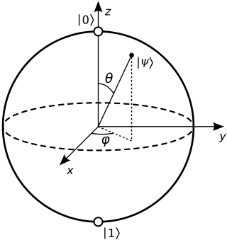
A general vector that points to any place on the surface is written as a ket ${\displaystyle |\psi \rangle }$. When employing the Poincaré sphere (also known as the Bloch sphere), the basis kets (${\displaystyle |0\rangle }$ and ${\displaystyle |1\rangle }$) must be assigned to opposing (antipodal) pairs of the kets listed above. For example, one might assign ${\displaystyle |0\rangle }$ = ${\displaystyle |H\rangle }$ and ${\displaystyle |1\rangle }$ = ${\displaystyle |V\rangle }$. These assignments are arbitrary. Opposing pairs are

• ${\displaystyle |H\rangle }$ and ${\displaystyle |V\rangle }$
• ${\displaystyle |D\rangle }$ and ${\displaystyle |A\rangle }$
• ${\displaystyle |R\rangle }$ and ${\displaystyle |L\rangle }$

The polarization of any point not equal to ${\displaystyle |R\rangle }$ or ${\displaystyle |L\rangle }$ and not on the circle that passes through ${\displaystyle |H\rangle ,|D\rangle ,|V\rangle ,|A\rangle }$ is known as elliptical polarization.

Jones matrices

The Jones matrices are operators that act on the Jones vectors defined above. These matrices are implemented by various optical elements such as lenses, beam splitters, mirrors, etc. Each matrix represents projection onto a one-dimensional complex subspace of the Jones vectors. The following table gives examples of Jones matrices for polarizers:

Optical element	Jones matrix
Linear polarizer with axis of transmission horizontal [2]	${\displaystyle {\begin{pmatrix}1&0\\0&0\end{pmatrix}}}$
Linear polarizer with axis of transmission vertical [2]	${\displaystyle {\begin{pmatrix}0&0\\0&1\end{pmatrix}}}$
Linear polarizer with axis of transmission at ±45° with the horizontal [2]	${\displaystyle {\frac {1}{2}}{\begin{pmatrix}1&\pm 1\\\pm 1&1\end{pmatrix}}}$
Linear polarizer with axis of transmission angle ${\displaystyle \theta }$ from the horizontal [2]	${\displaystyle {\begin{pmatrix}\cos ^{2}(\theta )&\cos(\theta )\sin(\theta )\\\cos(\theta )\sin(\theta )&\sin ^{2}(\theta )\end{pmatrix}}}$
Right circular polarizer [2]	${\displaystyle {\frac {1}{2}}{\begin{pmatrix}1&i\\-i&1\end{pmatrix}}}$
Left circular polarizer [2]	${\displaystyle {\frac {1}{2}}{\begin{pmatrix}1&-i\\i&1\end{pmatrix}}}$

Phase retarders

A phase retarder is an optical element that produces a phase difference between two orthogonal polarization components of a monochromatic polarized beam of light. ^[3] Mathematically, using kets to represent Jones vectors, this means that the action of a phase retarder is to transform light with polarization

${\displaystyle |P\rangle =c_{1}|1\rangle +c_{2}|2\rangle }$

to

${\displaystyle |P'\rangle =c_{1}{\rm {e}}^{i\eta /2}|1\rangle +c_{2}{\rm {e}}^{-i\eta /2}|2\rangle }$

where ${\displaystyle |1\rangle ,|2\rangle }$ are orthogonal polarization components (i.e. ${\displaystyle \langle 1|2\rangle =0}$) that are determined by the physical nature of the phase retarder. In general, the orthogonal components could be any two basis vectors. For example, the action of the circular phase retarder is such that

${\displaystyle |1\rangle ={\frac {1}{\sqrt {2}}}{\begin{pmatrix}1\\-i\end{pmatrix}}\qquad {\text{ and }}\qquad |2\rangle ={\frac {1}{\sqrt {2}}}{\begin{pmatrix}1\\i\end{pmatrix}}}$

However, linear phase retarders, for which ${\displaystyle |1\rangle ,|2\rangle }$ are linear polarizations, are more commonly encountered in discussion and in practice. In fact, sometimes the term "phase retarder" is used to refer specifically to linear phase retarders.

Linear phase retarders are usually made out of birefringent uniaxial crystals such as calcite, MgF₂ or quartz. Plates made of these materials for this purpose are referred to as waveplates. Uniaxial crystals have one crystal axis that is different from the other two crystal axes (i.e., n_i ≠ n_j = n_k). This unique axis is called the extraordinary axis and is also referred to as the optic axis. An optic axis can be the fast or the slow axis for the crystal depending on the crystal at hand. Light travels with a higher phase velocity along an axis that has the smallest refractive index and this axis is called the fast axis. Similarly, an axis which has the largest refractive index is called a slow axis since the phase velocity of light is the lowest along this axis. "Negative" uniaxial crystals (e.g., calcite CaCO₃, sapphire Al₂O₃) have n_e < n_o so for these crystals, the extraordinary axis (optic axis) is the fast axis, whereas for "positive" uniaxial crystals (e.g., quartz SiO₂, magnesium fluoride MgF₂, rutile TiO₂), n_e > n_o and thus the extraordinary axis (optic axis) is the slow axis. Other commercially available linear phase retarders exist and are used in more specialized applications. The Fresnel rhombs is one such alternative.

Any linear phase retarder with its fast axis defined as the x- or y-axis has zero off-diagonal terms and thus can be conveniently expressed as

${\displaystyle {\begin{pmatrix}{\rm {e}}^{i\phi _{x}}&0\\0&{\rm {e}}^{i\phi _{y}}\end{pmatrix}}}$

where ${\displaystyle \phi _{x}}$ and ${\displaystyle \phi _{y}}$ are the phase offsets of the electric fields in ${\displaystyle x}$ and ${\displaystyle y}$ directions respectively. In the phase convention ${\displaystyle \phi =kz-\omega t}$, define the relative phase between the two waves as ${\displaystyle \epsilon =\phi _{y}-\phi _{x}}$. Then a positive ${\displaystyle \epsilon }$ (i.e. ${\displaystyle \phi _{y}}$ > ${\displaystyle \phi _{x}}$) means that ${\displaystyle E_{y}}$ doesn't attain the same value as ${\displaystyle E_{x}}$ until a later time, i.e. ${\displaystyle E_{x}}$ leads ${\displaystyle E_{y}}$. Similarly, if ${\displaystyle \epsilon <0}$, then ${\displaystyle E_{y}}$ leads ${\displaystyle E_{x}}$.

For example, if the fast axis of a quarter waveplate is horizontal, then the phase velocity along the horizontal direction is ahead of the vertical direction i.e., ${\displaystyle E_{x}}$ leads ${\displaystyle E_{y}}$. Thus, ${\displaystyle \phi _{x}<\phi _{y}}$ which for a quarter waveplate yields ${\displaystyle \phi _{y}=\phi _{x}+\pi /2}$.

In the opposite convention ${\displaystyle \phi =\omega t-kz}$, define the relative phase as ${\displaystyle \epsilon =\phi _{x}-\phi _{y}}$. Then ${\displaystyle \epsilon >0}$ means that ${\displaystyle E_{y}}$ doesn't attain the same value as ${\displaystyle E_{x}}$ until a later time, i.e. ${\displaystyle E_{x}}$ leads ${\displaystyle E_{y}}$.

Phase retarders	Corresponding Jones matrix
Quarter-wave plate with fast axis vertical [4] [note 1]	${\displaystyle {\rm {e}}^{\frac {i\pi }{4}}{\begin{pmatrix}1&0\\0&-i\end{pmatrix}}}$
Quarter-wave plate with fast axis horizontal [4]	${\displaystyle {\rm {e}}^{-{\frac {i\pi }{4}}}{\begin{pmatrix}1&0\\0&i\end{pmatrix}}}$
Quarter-wave plate with fast axis at angle ${\displaystyle \theta }$ w.r.t the horizontal axis	${\displaystyle {\rm {e}}^{-{\frac {i\pi }{4}}}{\begin{pmatrix}\cos ^{2}\theta +i\sin ^{2}\theta &(1-i)\sin \theta \cos \theta \\(1-i)\sin \theta \cos \theta &\sin ^{2}\theta +i\cos ^{2}\theta \end{pmatrix}}}$
Half-wave plate rotated by ${\displaystyle \theta }$ [5]	${\displaystyle {\begin{pmatrix}\cos 2\theta &\sin 2\theta \\\sin 2\theta &-\cos 2\theta \end{pmatrix}}}$
Half-wave plate with fast axis at angle ${\displaystyle \theta }$ w.r.t the horizontal axis [6]	${\displaystyle {\rm {e}}^{-{\frac {i\pi }{2}}}{\begin{pmatrix}\cos ^{2}\theta -\sin ^{2}\theta &2\cos \theta \sin \theta \\2\cos \theta \sin \theta &\sin ^{2}\theta -\cos ^{2}\theta \end{pmatrix}}}$
General Waveplate (Linear Phase Retarder) [3]	${\displaystyle {\rm {e}}^{-{\frac {i\eta }{2}}}{\begin{pmatrix}\cos ^{2}\theta +{\rm {e}}^{i\eta }\sin ^{2}\theta &\left(1-{\rm {e}}^{i\eta }\right)\cos \theta \sin \theta \\\left(1-{\rm {e}}^{i\eta }\right)\cos \theta \sin \theta &\sin ^{2}\theta +{\rm {e}}^{i\eta }\cos ^{2}\theta \end{pmatrix}}}$
Arbitrary birefringent material (Elliptical phase retarder) [3] [7]	${\displaystyle {\rm {e}}^{-{\frac {i\eta }{2}}}{\begin{pmatrix}\cos ^{2}\theta +{\rm {e}}^{i\eta }\sin ^{2}\theta &\left(1-{\rm {e}}^{i\eta }\right){\rm {e}}^{-i\phi }\cos \theta \sin \theta \\\left(1-{\rm {e}}^{i\eta }\right){\rm {e}}^{i\phi }\cos \theta \sin \theta &\sin ^{2}\theta +{\rm {e}}^{i\eta }\cos ^{2}\theta \end{pmatrix}}}$

The Jones matrix for an arbitrary birefringent material is the most general form of a polarization transformation in the Jones calculus; it can represent any polarization transformation. To see this, one can show

${\displaystyle {\begin{aligned}&{\rm {e}}^{-{\frac {i\eta }{2}}}{\begin{pmatrix}\cos ^{2}\theta +{\rm {e}}^{i\eta }\sin ^{2}\theta &\left(1-{\rm {e}}^{i\eta }\right){\rm {e}}^{-i\phi }\cos \theta \sin \theta \\\left(1-{\rm {e}}^{i\eta }\right){\rm {e}}^{i\phi }\cos \theta \sin \theta &\sin ^{2}\theta +{\rm {e}}^{i\eta }\cos ^{2}\theta \end{pmatrix}}\\&={\begin{pmatrix}\cos(\eta /2)-i\sin(\eta /2)\cos(2\theta )&-\sin(\eta /2)\sin(\phi )\sin(2\theta )-i\sin(\eta /2)\cos(\phi )\sin(2\theta )\\\sin(\eta /2)\sin(\phi )\sin(2\theta )-i\sin(\eta /2)\cos(\phi )\sin(2\theta )&\cos(\eta /2)+i\sin(\eta /2)\cos(2\theta )\end{pmatrix}}\end{aligned}}}$

The above matrix is a general parametrization for the elements of SU(2), using the convention

${\displaystyle \operatorname {SU} (2)=\left\{{\begin{pmatrix}\alpha &-{\overline {\beta }}\\\beta &{\overline {\alpha }}\end{pmatrix}}:\ \ \alpha ,\beta \in \mathbb {C} ,\ \ |\alpha |^{2}+|\beta |^{2}=1\right\}~}$

where the overline denotes complex conjugation.

Finally, recognizing that the set of unitary transformations on ${\displaystyle \mathbb {C} ^{2}}$ can be expressed as

${\displaystyle \left\{{\rm {e}}^{i\gamma }{\begin{pmatrix}\alpha &-{\overline {\beta }}\\\beta &{\overline {\alpha }}\end{pmatrix}}:\ \ \alpha ,\beta \in \mathbb {C} ,\ \ |\alpha |^{2}+|\beta |^{2}=1,\ \ \gamma \in [0,2\pi ]\right\}}$

it becomes clear that the Jones matrix for an arbitrary birefringent material represents any unitary transformation, up to a phase factor ${\displaystyle {\rm {e}}^{i\gamma }}$. Therefore, for appropriate choice of ${\displaystyle \eta }$, ${\displaystyle \theta }$, and ${\displaystyle \phi }$, a transformation between any two Jones vectors can be found, up to a phase factor ${\displaystyle {\rm {e}}^{i\gamma }}$. However, in the Jones calculus, such phase factors do not change the represented polarization of a Jones vector, so are either considered arbitrary or imposed ad hoc to conform to a set convention.

The special expressions for the phase retarders can be obtained by taking suitable parameter values in the general expression for a birefringent material. ^[7] In the general expression:

• The relative phase retardation induced between the fast axis and the slow axis is given by ${\displaystyle \eta =\phi _{y}-\phi _{x}}$
• ${\displaystyle \theta }$ is the orientation of the fast axis with respect to the x-axis.
• ${\displaystyle \phi }$ is the circularity.

Note that for linear retarders, ${\displaystyle \phi }$ = 0 and for circular retarders, ${\displaystyle \phi }$ = ± ${\displaystyle \pi }$/2, ${\displaystyle \theta }$ = ${\displaystyle \pi }$/4. In general for elliptical retarders, ${\displaystyle \phi }$ takes on values between - ${\displaystyle \pi }$/2 and ${\displaystyle \pi }$/2.

Axially rotated elements

Assume an optical element has its optic axis^{[ clarification needed ]} perpendicular to the surface vector for the plane of incidence ^{[ clarification needed ]} and is rotated about this surface vector by angle θ/2 (i.e., the principal plane through which the optic axis passes,^{[ clarification needed ]} makes angle θ/2 with respect to the plane of polarization of the electric field^{[ clarification needed ]} of the incident TE wave). Recall that a half-wave plate rotates polarization as twice the angle between incident polarization and optic axis (principal plane). Therefore, the Jones matrix for the rotated polarization state, M(θ), is

${\displaystyle M(\theta )=R(-\theta )\,M\,R(\theta ),}$

where ${\displaystyle R(\theta )={\begin{pmatrix}\cos \theta &\sin \theta \\-\sin \theta &\cos \theta \end{pmatrix}}.}$

This agrees with the expression for a half-wave plate in the table above. These rotations are identical to beam unitary splitter transformation in optical physics given by

${\displaystyle R(\theta )={\begin{pmatrix}r&t'\\t&r'\end{pmatrix}}}$

where the primed and unprimed coefficients represent beams incident from opposite sides of the beam splitter. The reflected and transmitted components acquire a phase θ_r and θ_t, respectively. The requirements for a valid representation of the element are ^[8]

${\displaystyle \theta _{\text{t}}-\theta _{\text{r}}+\theta _{\text{t'}}-\theta _{\text{r'}}=\pm \pi }$

and ${\displaystyle r^{*}t'+t^{*}r'=0.}$

Both of these representations are unitary matrices fitting these requirements; and as such, are both valid.

Arbitrarily rotated elements

This would involve a three-dimensional rotation matrix. See Russell A. Chipman and Garam Yun for work done on this. ^{[9] [10] [11] [12]}

See also

• Polarization
• Scattering parameters
• Stokes parameters
• Mueller calculus
• Photon polarization

Notes

1. The prefactor ${\displaystyle {\rm {e}}^{i\pi /4}}$ appears only if one defines the phase delays in a symmetric fashion; that is, ${\displaystyle \phi _{x}=-\phi _{y}=\pi /4}$. This is done in Hecht ^[4] but not in Fowles. ^[2] In the latter reference the Jones matrices for a quarter-wave plate have no prefactor.

References

1. "Jones Calculus". spie.org. Retrieved 2022-08-07.
2. Fowles, G. (1989). Introduction to Modern Optics (2nd ed.). Dover. p.  35. ISBN   9780486659572.
3. P.S. Theocaris; E.E. Gdoutos (1979). Matrix Theory of Photoelasticity. Springer Series in Optical Sciences. Vol. 11 (1st ed.). Springer-Verlag. doi:10.1007/978-3-540-35789-6. ISBN   978-3-662-15807-4.
4. Eugene Hecht (2001). Optics (4th ed.). p.  378. ISBN   978-0805385663.
5. "Jones Calculus". spie.org. Retrieved 2023-04-29.
6. Gerald, A.; Burch, J.M. (1975). Introduction to Matrix Methods in Optics (1st ed.). John Wiley & Sons. p. 212. ISBN   978-0471296850.
7. Gill, Jose Jorge; Bernabeu, Eusebio (1987). "Obtainment of the polarizing and retardation parameters of a non-depolarizing optical system from the polar decomposition of its Mueller matrix". Optik . 76 (2): 67–71. ISSN   0030-4026.
8. Ou, Z. Y.; Mandel, L. (1989). "Derivation of reciprocity relations for a beam splitter from energy balance". Am. J. Phys. 57 (1): 66. Bibcode:1989AmJPh..57...66O. doi:10.1119/1.15873.
9. Chipman, Russell A. (1995). "Mechanics of polarization ray tracing". Opt. Eng. 34 (6): 1636–1645. Bibcode:1995OptEn..34.1636C. doi:10.1117/12.202061.
10. Yun, Garam; Crabtree, Karlton; Chipman, Russell A. (2011). "Three-dimensional polarization ray-tracing calculus I: definition and diattenuation". Applied Optics . 50 (18): 2855–2865. Bibcode:2011ApOpt..50.2855Y. doi:10.1364/AO.50.002855. PMID   21691348.
11. Yun, Garam; McClain, Stephen C.; Chipman, Russell A. (2011). "Three-dimensional polarization ray-tracing calculus II: retardance". Applied Optics. 50 (18): 2866–2874. Bibcode:2011ApOpt..50.2866Y. doi:10.1364/AO.50.002866. PMID   21691349.
12. Yun, Garam (2011). Polarization Ray Tracing (PhD thesis). University of Arizona. hdl:10150/202979.

Further reading

• E. Collett, Field Guide to Polarization, SPIE Field Guides vol. FG05, SPIE (2005). ISBN   0-8194-5868-6.
• D. Goldstein and E. Collett, Polarized Light, 2nd ed., CRC Press (2003). ISBN   0-8247-4053-X.
• E. Hecht, Optics, 2nd ed., Addison-Wesley (1987). ISBN   0-201-11609-X.
• Frank L. Pedrotti, S.J. Leno S. Pedrotti, Introduction to Optics, 2nd ed., Prentice Hall (1993). ISBN   0-13-501545-6
• A. Gerald and J.M. Burch, Introduction to Matrix Methods in Optics,1st ed., John Wiley & Sons(1975). ISBN   0-471-29685-6
• Jones, R. Clark (1941). "A new calculus for the treatment of optical systems, I. Description and Discussion of the Calculus". Journal of the Optical Society of America. 31 (7): 488–493. doi:10.1364/JOSA.31.000488.
• Hurwitz, Henry; Jones, R. Clark (1941). "A new calculus for the treatment of optical systems, II. Proof of three general equivalence theorems". Journal of the Optical Society of America. 31 (7): 493–499. doi:10.1364/JOSA.31.000493.
• Jones, R. Clark (1941). "A new calculus for the treatment of optical systems, III The Sohncke Theory of optical activity". Journal of the Optical Society of America. 31 (7): 500–503. doi:10.1364/JOSA.31.000500.
• Jones, R. Clark (1942). "A new calculus for the treatment of optical systems, IV". Journal of the Optical Society of America. 32 (8): 486–493. doi:10.1364/JOSA.32.000486.
• Fymat, A. L. (1971). "Jones's Matrix Representation of Optical Instruments. I: Beam Splitters". Applied Optics. 10 (11): 2499–2505. Bibcode:1971ApOpt..10.2499F. doi:10.1364/AO.10.002499. PMID   20111363.
• Fymat, A. L. (1971). "Jones's Matrix Representation of Optical Instruments. 2: Fourier Interferometers (Spectrometers and Spectropolarimeters)". Applied Optics. 10 (12): 2711–2716. Bibcode:1971ApOpt..10.2711F. doi:10.1364/AO.10.002711. PMID   20111418.
• Fymat, A. L. (1972). "Polarization Effects in Fourier Spectroscopy. I: Coherency Matrix Representation". Applied Optics. 11 (1): 160–173. Bibcode:1972ApOpt..11..160F. doi:10.1364/AO.11.000160. PMID   20111472.
• Gill, Jose Jorge; Bernabeu, Eusebio (1987). "Obtainment of the polarizing and retardation parameters of a non-depolarizing optical system from the polar decomposition of its Mueller matrix". Optik. 76: 67–71.
• Brosseau, Christian; Givens, Clark R.; Kostinski, Alexander B. (1993). "Generalized trace condition on the Mueller-Jones polarization matrix". Journal of the Optical Society of America A. 10 (10): 2248–2251. Bibcode:1993JOSAA..10.2248B. doi:10.1364/JOSAA.10.002248.
• McGuire, James P.; Chipman, Russel A. (1994). "Polarization aberrations. 1. Rotationally symmetric optical systems". Applied Optics. 33 (22): 5080–5100. Bibcode:1994ApOpt..33.5080M. doi:10.1364/AO.33.005080. PMID   20935891. S2CID   3805982.
• Pistoni, Natale C. (1995). "Simplified approach to the Jones calculus in retracing optical circuits". Applied Optics. 34 (34): 7870–7876. Bibcode:1995ApOpt..34.7870P. doi:10.1364/AO.34.007870. PMID   21068881.
• Moreno, Ignacio; Yzuel, Maria J.; Campos, Juan; Vargas, Asticio (2004). "Jones matrix treatment for polarization Fourier optics". Journal of Modern Optics. 51 (14): 2031–2038. Bibcode:2004JMOp...51.2031M. doi:10.1080/09500340408232511. hdl: 10533/175322 . S2CID   120169144.
• Moreno, Ivan (2004). "Jones matrix for image-rotation prisms". Applied Optics. 43 (17): 3373–3381. Bibcode:2004ApOpt..43.3373M. doi:10.1364/AO.43.003373. PMID   15219016. S2CID   24268298.
• William Shurcliff (1966) Polarized Light: Production and Use, chapter 8 Mueller Calculus and Jones Calculus, page 109, Harvard University Press.

External links

• Jones Calculus written by E. Collett on Optipedia