Leading-order term

Last updated

The leading-order terms (or corrections) within a mathematical equation, expression or model are the terms with the largest order of magnitude. [1] [2] The sizes of the different terms in the equation(s) will change as the variables change, and hence, which terms are leading-order may also change.

Contents

A common and powerful way of simplifying and understanding a wide variety of complicated mathematical models is to investigate which terms are the largest (and therefore most important), for particular sizes of the variables and parameters, and analyse the behaviour produced by just these terms (regarding the other smaller terms as negligible). [3] [4] This gives the main behaviour – the true behaviour is only small deviations away from this. This main behaviour may be captured sufficiently well by just the strictly leading-order terms, or it may be decided that slightly smaller terms should also be included. In which case, the phrase leading-order terms might be used informally to mean this whole group of terms. The behaviour produced by just the group of leading-order terms is called the leading-order behaviour of the model.

Basic example

Sizes of the individual terms in y = x3 + 5x + 0.1. (Leading-order terms highlighted in pink.)
x0.0010.10.5210
x30.0000000010.0010.12581000
5x0.0050.52.51050
0.10.10.10.10.10.1
y0.1050000010.6012.72518.11050.1

Consider the equation y = x3 + 5x + 0.1. For five different values of x, the table shows the sizes of the four terms in this equation, and which terms are leading-order. As x increases further, the leading-order terms stay as x3 and y, but as x decreases and then becomes more and more negative, which terms are leading-order again changes.

There is no strict cut-off for when two terms should or should not be regarded as approximately the same order, or magnitude. One possible rule of thumb is that two terms that are within a factor of 10 (one order of magnitude) of each other should be regarded as of about the same order, and two terms that are not within a factor of 100 (two orders of magnitude) of each other should not. However, in between is a grey area, so there are no fixed boundaries where terms are to be regarded as approximately leading-order and where not. Instead the terms fade in and out, as the variables change. Deciding whether terms in a model are leading-order (or approximately leading-order), and if not, whether they are small enough to be regarded as negligible, (two different questions), is often a matter of investigation and judgement, and will depend on the context.

Leading-order behaviour

Equations with only one leading-order term are possible, but rare.[ dubious ] For example, the equation 100 = 1 + 1 + 1 + ... + 1, (where the right hand side comprises one hundred 1's). For any particular combination of values for the variables and parameters, an equation will typically contain at least two leading-order terms, and other lower-order terms. In this case, by making the assumption that the lower-order terms, and the parts of the leading-order terms that are the same size as the lower-order terms (perhaps the second or third significant figure onwards), are negligible, a new equation may be formed by dropping all these lower-order terms and parts of the leading-order terms. The remaining terms provide the leading-order equation, or leading-order balance, [5] or dominant balance, [6] [7] [8] and creating a new equation just involving these terms is known as taking an equation to leading-order. The solutions to this new equation are called the leading-order solutions [9] [10] to the original equation. Analysing the behaviour given by this new equation gives the leading-order behaviour [11] [12] of the model for these values of the variables and parameters. The size of the error in making this approximation is normally roughly the size of the largest neglected term.

Graph of y = x + 5x + 0.1. The leading order, or main, behaviour at x = 0.001 is that y is constant, and at x = 10 is that y increases cubically with x. LeadingOrderGraph.JPG
Graph of y = x + 5x + 0.1. The leading order, or main, behaviour at x = 0.001 is that y is constant, and at x = 10 is that y increases cubically with x.

Suppose we want to understand the leading-order behaviour of the example above.

The main behaviour of y may thus be investigated at any value of x. The leading-order behaviour is more complicated when more terms are leading-order. At x=2 there is a leading-order balance between the cubic and linear dependencies of y on x.

Note that this description of finding leading-order balances and behaviours gives only an outline description of the process – it is not mathematically rigorous.

Next-to-leading order

Of course, y is not actually completely constant at x = 0.001 – this is just its main behaviour in the vicinity of this point. It may be that retaining only the leading-order (or approximately leading-order) terms, and regarding all the other smaller terms as negligible, is insufficient (when using the model for future prediction, for example), and so it may be necessary to also retain the set of next largest terms. These can be called the next-to-leading order (NLO) terms or corrections. [13] [14] The next set of terms down after that can be called the next-to-next-to-leading order (NNLO) terms or corrections. [15]

Usage

Matched asymptotic expansions

Leading-order simplification techniques are used in conjunction with the method of matched asymptotic expansions, when the accurate approximate solution in each subdomain is the leading-order solution. [3] [16] [17]

Simplifying the Navier–Stokes equations

For particular fluid flow scenarios, the (very general) Navier–Stokes equations may be considerably simplified by considering only the leading-order components. For example, the Stokes flow equations. [18] Also, the thin film equations of lubrication theory.

Simplification of differential equations by machine learning

Various differential equations may be locally simplified by considering only the leading-order components. Machine learning algorithms can partition simulation or observational data into localized partitions with leading-order equation terms for aerodynamics, ocean dynamics, tumor-induced angiogenesis, and synthetic data applications. [19]

See also

Related Research Articles

In physics, quintessence is a hypothetical form of dark energy, more precisely a scalar field, postulated as an explanation of the observation of an accelerating rate of expansion of the universe. The first example of this scenario was proposed by Ratra and Peebles (1988) and Wetterich (1988). The concept was expanded to more general types of time-varying dark energy, and the term "quintessence" was first introduced in a 1998 paper by Robert R. Caldwell, Rahul Dave and Paul Steinhardt. It has been proposed by some physicists to be a fifth fundamental force. Quintessence differs from the cosmological constant explanation of dark energy in that it is dynamic; that is, it changes over time, unlike the cosmological constant which, by definition, does not change. Quintessence can be either attractive or repulsive depending on the ratio of its kinetic and potential energy. Those working with this postulate believe that quintessence became repulsive about ten billion years ago, about 3.5 billion years after the Big Bang.

<span class="mw-page-title-main">Positronium</span> Bound state of an electron and positron

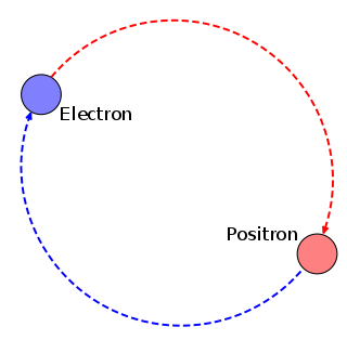
Positronium (Ps) is a system consisting of an electron and its anti-particle, a positron, bound together into an exotic atom, specifically an onium. Unlike hydrogen, the system has no protons. The system is unstable: the two particles annihilate each other to predominantly produce two or three gamma-rays, depending on the relative spin states. The energy levels of the two particles are similar to that of the hydrogen atom. However, because of the reduced mass, the frequencies of the spectral lines are less than half of those for the corresponding hydrogen lines.

<span class="mw-page-title-main">Top quark</span> Type of quark

The top quark, sometimes also referred to as the truth quark, is the most massive of all observed elementary particles. It derives its mass from its coupling to the Higgs Boson. This coupling is very close to unity; in the Standard Model of particle physics, it is the largest (strongest) coupling at the scale of the weak interactions and above. The top quark was discovered in 1995 by the CDF and DØ experiments at Fermilab.

<span class="mw-page-title-main">Technicolor (physics)</span> Hypothetical model through which W and Z bosons acquire mass

Technicolor theories are models of physics beyond the Standard Model that address electroweak gauge symmetry breaking, the mechanism through which W and Z bosons acquire masses. Early technicolor theories were modelled on quantum chromodynamics (QCD), the "color" theory of the strong nuclear force, which inspired their name.

In physics, mirror matter, also called shadow matter or Alice matter, is a hypothetical counterpart to ordinary matter.

In particle physics, the hypothetical dilaton particle is a particle of a scalar field that appears in theories with extra dimensions when the volume of the compactified dimensions varies. It appears as a radion in Kaluza–Klein theory's compactifications of extra dimensions. In Brans–Dicke theory of gravity, Newton's constant is not presumed to be constant but instead 1/G is replaced by a scalar field and the associated particle is the dilaton.

<span class="mw-page-title-main">Hierarchy problem</span> Unsolved problem in physics

In theoretical physics, the hierarchy problem is the problem concerning the large discrepancy between aspects of the weak force and gravity. There is no scientific consensus on why, for example, the weak force is 1024 times stronger than gravity.

In quantum electrodynamics, the anomalous magnetic moment of a particle is a contribution of effects of quantum mechanics, expressed by Feynman diagrams with loops, to the magnetic moment of that particle. The magnetic moment, also called magnetic dipole moment, is a measure of the strength of a magnetic source.

In mathematical physics, a caloron is the finite temperature generalization of an instanton.

Objective-collapse theories, also known as models of spontaneous wave function collapse or dynamical reduction models, are proposed solutions to the measurement problem in quantum mechanics. As with other theories called interpretations of quantum mechanics, they are possible explanations of why and how quantum measurements always give definite outcomes, not a superposition of them as predicted by the Schrödinger equation, and more generally how the classical world emerges from quantum theory. The fundamental idea is that the unitary evolution of the wave function describing the state of a quantum system is approximate. It works well for microscopic systems, but progressively loses its validity when the mass / complexity of the system increases.

<span class="mw-page-title-main">Christopher T. Hill</span> American theoretical physicist

Christopher T. Hill is an American theoretical physicist at the Fermi National Accelerator Laboratory who did undergraduate work in physics at M.I.T., and graduate work at Caltech. Hill's Ph.D. thesis, "Higgs Scalars and the Nonleptonic Weak Interactions" (1977) contains one of the first detailed discussions of the two-Higgs-doublet model and its impact upon weak interactions.

In particle physics and string theory (M-theory), the ADD model, also known as the model with large extra dimensions (LED), is a model framework that attempts to solve the hierarchy problem. The model tries to explain this problem by postulating that our universe, with its four dimensions, exists on a membrane in a higher dimensional space. It is then suggested that the other forces of nature operate within this membrane and its four dimensions, while the hypothetical gravity-bearing particle graviton can propagate across the extra dimensions. This would explain why gravity is very weak compared to the other fundamental forces. The size of the dimensions in ADD is around the order of the TeV scale, which results in it being experimentally probeable by current colliders, unlike many exotic extra dimensional hypotheses that have the relevant size around the Planck scale.

<span class="mw-page-title-main">Light front quantization</span> Technique in computational quantum field theory

The light-front quantization of quantum field theories provides a useful alternative to ordinary equal-time quantization. In particular, it can lead to a relativistic description of bound systems in terms of quantum-mechanical wave functions. The quantization is based on the choice of light-front coordinates, where plays the role of time and the corresponding spatial coordinate is . Here, is the ordinary time, is one Cartesian coordinate, and is the speed of light. The other two Cartesian coordinates, and , are untouched and often called transverse or perpendicular, denoted by symbols of the type . The choice of the frame of reference where the time and -axis are defined can be left unspecified in an exactly soluble relativistic theory, but in practical calculations some choices may be more suitable than others.

Thomas Carlos Mehen is an American physicist. His research has consisted of primarily Quantum chromodynamics (QCD) and the application of effective field theory to problems in hadronic physics. He has also worked on effective field theory for non-relativistic particles whose short range interactions are characterized by a large scattering length, as well as novel field theories which arise from unusual limits of string theory.

In particle physics, W′ and Z′ bosons refer to hypothetical gauge bosons that arise from extensions of the electroweak symmetry of the Standard Model. They are named in analogy with the Standard Model W and Z bosons.

<span class="mw-page-title-main">Light front holography</span> Technique used to determine mass of hadrons

In strong interaction physics, light front holography or light front holographic QCD is an approximate version of the theory of quantum chromodynamics (QCD) which results from mapping the gauge theory of QCD to a higher-dimensional anti-de Sitter space (AdS) inspired by the AdS/CFT correspondence proposed for string theory. This procedure makes it possible to find analytic solutions in situations where strong coupling occurs, improving predictions of the masses of hadrons and their internal structure revealed by high-energy accelerator experiments. The most widely used approach to finding approximate solutions to the QCD equations, lattice QCD, has had many successful applications; however, it is a numerical approach formulated in Euclidean space rather than physical Minkowski space-time.

<span class="mw-page-title-main">Light-front quantization applications</span> Quantization procedure in quantum field theory

The light-front quantization of quantum field theories provides a useful alternative to ordinary equal-time quantization. In particular, it can lead to a relativistic description of bound systems in terms of quantum-mechanical wave functions. The quantization is based on the choice of light-front coordinates, where plays the role of time and the corresponding spatial coordinate is . Here, is the ordinary time, is a Cartesian coordinate, and is the speed of light. The other two Cartesian coordinates, and , are untouched and often called transverse or perpendicular, denoted by symbols of the type . The choice of the frame of reference where the time and -axis are defined can be left unspecified in an exactly soluble relativistic theory, but in practical calculations some choices may be more suitable than others. The basic formalism is discussed elsewhere.

<span class="mw-page-title-main">Light-front computational methods</span> Technique in computational quantum field theory

The light-front quantization of quantum field theories provides a useful alternative to ordinary equal-time quantization. In particular, it can lead to a relativistic description of bound systems in terms of quantum-mechanical wave functions. The quantization is based on the choice of light-front coordinates, where plays the role of time and the corresponding spatial coordinate is . Here, is the ordinary time, is one Cartesian coordinate, and is the speed of light. The other two Cartesian coordinates, and , are untouched and often called transverse or perpendicular, denoted by symbols of the type . The choice of the frame of reference where the time and -axis are defined can be left unspecified in an exactly soluble relativistic theory, but in practical calculations some choices may be more suitable than others.

The Kundu equation is a general form of integrable system that is gauge-equivalent to the mixed nonlinear Schrödinger equation. It was proposed by Anjan Kundu as

Starobinsky inflation is a modification of general relativity used to explain cosmological inflation.

References

  1. J.K.Hunter, Asymptotic Analysis and Singular Perturbation Theory, 2004. http://www.math.ucdavis.edu/~hunter/notes/asy.pdf
  2. NYU course notes
  3. 1 2 Mitchell, M. J.; et al. (2010). "A model of carbon dioxide dissolution and mineral carbonation kinetics". Proceedings of the Royal Society A . 466 (2117): 1265–1290. Bibcode:2010RSPSA.466.1265M. doi: 10.1098/rspa.2009.0349 .
  4. Woollard, H. F.; et al. (2008). "A multi-scale model for solute transport in a wavy-walled channel" (PDF). Journal of Engineering Mathematics. 64 (1): 25–48. Bibcode:2009JEnMa..64...25W. doi: 10.1007/s10665-008-9239-x .
  5. Sternberg, P.; Bernoff, A. J. (1998). "Onset of Superconductivity in Decreasing Fields for General Domains". Journal of Mathematical Physics. 39 (3): 1272–1284. Bibcode:1998JMP....39.1272B. doi:10.1063/1.532379.
  6. Salamon, T.R.; et al. (1995). "The role of surface tension in the dominant balance in the die swell singularity". Physics of Fluids. 7 (10): 2328–2344. Bibcode:1995PhFl....7.2328S. doi:10.1063/1.868746. Archived from the original on 2013-07-08.
  7. Gorshkov, A. V.; et al. (2008). "Coherent Quantum Optical Control with Subwavelength Resolution". Physical Review Letters. 100 (9): 93005. arXiv: 0706.3879 . Bibcode:2008PhRvL.100i3005G. doi:10.1103/PhysRevLett.100.093005. PMID   18352706. S2CID   3789664.
  8. Lindenberg, K.; et al. (1994). "Diffusion-Limited Binary Reactions: The Hierarchy of Nonclassical Regimes for Correlated Initial Conditions" (PDF). Journal of Physical Chemistry. 98 (13): 3389–3397. doi:10.1021/j100064a020.
  9. Żenczykowski, P. (1988). "Kobayashi–Maskawa matrix from the leading-order solution of the n-generation Fritzsch model". Physical Review D. 38 (1): 332–336. Bibcode:1988PhRvD..38..332Z. doi:10.1103/PhysRevD.38.332. PMID   9959017.
  10. Horowitz, G. T.; Tseytlin, A. A. (1994). "Extremal black holes as exact string solutions". Physical Review Letters. 73 (25): 3351–3354. arXiv: hep-th/9408040 . Bibcode:1994PhRvL..73.3351H. doi:10.1103/PhysRevLett.73.3351. PMID   10057359. S2CID   43551044.
  11. Hüseyin, A. (1980). "The leading-order behaviour of the two-photon scattering amplitudes in QCD". Nuclear Physics B. 163: 453–460. Bibcode:1980NuPhB.163..453A. doi:10.1016/0550-3213(80)90411-3.
  12. Kruczenski, M.; Oxman, L.E.; Zaldarriaga, M. (1999). "Large squeezing behaviour of cosmological entropy generation". Classical and Quantum Gravity. 11 (9): 2317–2329. arXiv: gr-qc/9403024 . Bibcode:1994CQGra..11.2317K. doi:10.1088/0264-9381/11/9/013. S2CID   13979794.
  13. Campbell, J.; Ellis, R.K. (2002). "Next-to-leading order corrections to W + 2 jet and Z + 2 jet production at hadron colliders". Physical Review D. 65 (11): 113007. arXiv: hep-ph/0202176 . Bibcode:2002PhRvD..65k3007C. doi:10.1103/PhysRevD.65.113007. S2CID   119355645.
  14. Catani, S.; Seymour, M.H. (1996). "The Dipole Formalism for the Calculation of QCD Jet Cross Sections at Next-to-Leading Order". Physics Letters B. 378 (1): 287–301. arXiv: hep-ph/9602277 . Bibcode:1996PhLB..378..287C. doi:10.1016/0370-2693(96)00425-X. S2CID   15422325.
  15. Kidonakis, N.; Vogt, R. (2003). "Next-to-next-to-leading order soft-gluon corrections in top quark hadroproduction". Physical Review D. 68 (11): 114014. arXiv: hep-ph/0308222 . Bibcode:2003PhRvD..68k4014K. doi:10.1103/PhysRevD.68.114014. S2CID   5943465.
  16. Rubinstein, B.Y.; Pismen, L.M. (1994). "Vortex motion in the spatially inhomogeneous conservative Ginzburg–Landau model" (PDF). Physica D: Nonlinear Phenomena. 78 (1): 1–10. Bibcode:1994PhyD...78....1R. doi:10.1016/0167-2789(94)00119-7.
  17. Kivshar, Y.S.; et al. (1998). "Dynamics of optical vortex solitons" (PDF). Optics Communications. 152 (1): 198–206. Bibcode:1998OptCo.152..198K. doi:10.1016/S0030-4018(98)00149-7. Archived from the original (PDF) on 2013-04-21. Retrieved 2012-10-31.
  18. Cornell University notes
  19. Kaiser, Bryan E.; Saenz, Juan A.; Sonnewald, Maike; Livescu, Daniel (2022). "Automated identification of dominant physical processes". Engineering Applications of Artificial Intelligence. 116: 105496. doi: 10.1016/j.engappai.2022.105496 . S2CID   252957864.