In mathematics, Legendre polynomials, named after Adrien-Marie Legendre (1782), are a system of complete and orthogonal polynomials with a vast number of mathematical properties and numerous applications. They can be defined in many ways, and the various definitions highlight different aspects as well as suggest generalizations and connections to different mathematical structures and physical and numerical applications.
Definition by construction as an orthogonal system
In this approach, the polynomials are defined as an orthogonal system with respect to the weight function over the interval . That is, is a polynomial of degree , such that
With the additional standardization condition , all the polynomials can be uniquely determined. We then start the construction process: is the only correctly standardized polynomial of degree 0. must be orthogonal to , leading to , and is determined by demanding orthogonality to and , and so on. is fixed by demanding orthogonality to all with . This gives conditions, which, along with the standardization fixes all coefficients in . With work, all the coefficients of every polynomial can be systematically determined, leading to the explicit representation in powers of given below.
This definition of the 's is the simplest one. It does not appeal to the theory of differential equations. Second, the completeness of the polynomials follows immediately from the completeness of the powers 1, . Finally, by defining them via orthogonality with respect to the most obvious weight function on a finite interval, it sets up the Legendre polynomials as one of the three classical orthogonal polynomial systems. The other two are the Laguerre polynomials, which are orthogonal over the half line , and the Hermite polynomials, orthogonal over the full line , with weight functions that are the most natural analytic functions that ensure convergence of all integrals.
Definition via generating function
The Legendre polynomials can also be defined as the coefficients in a formal expansion in powers of of the generating function[1]
(2)
The coefficient of is a polynomial in of degree with . Expanding up to gives
Expansion to higher orders gets increasingly cumbersome, but is possible to do systematically, and again leads to one of the explicit forms given below.
It is possible to obtain the higher 's without resorting to direct expansion of the Taylor series, however. Equation2 is differentiated with respect to t on both sides and rearranged to obtain
Replacing the quotient of the square root with its definition in Eq.2, and equating the coefficients of powers of t in the resulting expansion gives Bonnet’s recursion formula
This relation, along with the first two polynomials P0 and P1, allows all the rest to be generated recursively.
The generating function approach is directly connected to the multipole expansion in electrostatics, as explained below, and is how the polynomials were first defined by Legendre in 1782.
Definition via differential equation
A third definition is in terms of solutions to Legendre's differential equation:
(1)
This differential equation has regular singular points at x = ±1 so if a solution is sought using the standard Frobenius or power series method, a series about the origin will only converge for |x| < 1 in general. When n is an integer, the solution Pn(x) that is regular at x = 1 is also regular at x = −1, and the series for this solution terminates (i.e. it is a polynomial). The orthogonality and completeness of these solutions is best seen from the viewpoint of Sturm–Liouville theory. We rewrite the differential equation as an eigenvalue problem,
with the eigenvalue in lieu of . If we demand that the solution be regular at , the differential operator on the left is Hermitian. The eigenvalues are found to be of the form n(n + 1), with and the eigenfunctions are the . The orthogonality and completeness of this set of solutions follows at once from the larger framework of Sturm–Liouville theory.
The differential equation admits another, non-polynomial solution, the Legendre functions of the second kind. A two-parameter generalization of (Eq.1) is called Legendre's general differential equation, solved by the Associated Legendre polynomials. Legendre functions are solutions of Legendre's differential equation (generalized or not) with non-integer parameters.
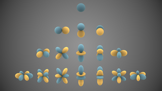
In physical settings, Legendre's differential equation arises naturally whenever one solves Laplace's equation (and related partial differential equations) by separation of variables in spherical coordinates. From this standpoint, the eigenfunctions of the angular part of the Laplacian operator are the spherical harmonics, of which the Legendre polynomials are (up to a multiplicative constant) the subset that is left invariant by rotations about the polar axis. The polynomials appear as where is the polar angle. This approach to the Legendre polynomials provides a deep connection to rotational symmetry. Many of their properties which are found laboriously through the methods of analysis — for example the addition theorem — are more easily found using the methods of symmetry and group theory, and acquire profound physical and geometrical meaning.
Orthogonality and completeness
The standardization fixes the normalization of the Legendre polynomials (with respect to the L2 norm on the interval −1 ≤ x ≤ 1). Since they are also orthogonal with respect to the same norm, the two statements[clarification needed] can be combined into the single equation,
(where δmn denotes the Kronecker delta, equal to 1 if m = n and to 0 otherwise). This normalization is most readily found by employing Rodrigues' formula, given below.
That the polynomials are complete means the following. Given any piecewise continuous function with finitely many discontinuities in the interval [−1, 1], the sequence of sums
converges in the mean to as , provided we take
This completeness property underlies all the expansions discussed in this article, and is often stated in the form
with −1 ≤ x ≤ 1 and −1 ≤ y ≤ 1.
Rodrigues' formula and other explicit formulas
An especially compact expression for the Legendre polynomials is given by Rodrigues' formula:
This formula enables derivation of a large number of properties of the 's. Among these are explicit representations such as
Expressing the polynomial as a power series, , the coefficients of powers of can also be calculated using a general formula:
The Legendre polynomial is determined by the values used for the two constants and , where if is odd and if is even.[2]
where r and r′ are the lengths of the vectors x and x′ respectively and γ is the angle between those two vectors. The series converges when r > r′. The expression gives the gravitational potential associated to a point mass or the Coulomb potential associated to a point charge. The expansion using Legendre polynomials might be useful, for instance, when integrating this expression over a continuous mass or charge distribution.
Legendre polynomials occur in the solution of Laplace's equation of the static potential, ∇2 Φ(x) = 0, in a charge-free region of space, using the method of separation of variables, where the boundary conditions have axial symmetry (no dependence on an azimuthal angle). Where ẑ is the axis of symmetry and θ is the angle between the position of the observer and the ẑ axis (the zenith angle), the solution for the potential will be
Al and Bl are to be determined according to the boundary condition of each problem.[4]
They also appear when solving the Schrödinger equation in three dimensions for a central force.
Legendre polynomials in multipole expansions
Diagram for the multipole expansion of electric potential.
Legendre polynomials are also useful in expanding functions of the form (this is the same as before, written a little differently):
If the radius r of the observation point P is greater than a, the potential may be expanded in the Legendre polynomials
where we have defined η = a/r < 1 and x = cos θ. This expansion is used to develop the normal multipole expansion.
Conversely, if the radius r of the observation point P is smaller than a, the potential may still be expanded in the Legendre polynomials as above, but with a and r exchanged. This expansion is the basis of interior multipole expansion.
Legendre polynomials in trigonometry
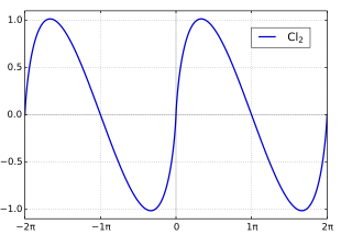
The trigonometric functions cos nθ, also denoted as the Chebyshev polynomialsTn(cos θ) ≡ cos nθ, can also be multipole expanded by the Legendre polynomials Pn(cos θ). The first several orders are as follows:
Another property is the expression for sin (n + 1)θ, which is
In this case, the sliding window of across the past units of time is best approximated by a linear combination of the first shifted Legendre polynomials, weighted together by the elements of at time :
When combined with deep learning methods, these networks can be trained to outperform long short-term memory units and related architectures, while using fewer computational resources.[5]
Additional properties of Legendre polynomials
Legendre polynomials have definite parity. That is, they are even or odd,[6] according to
Another useful property is
which follows from considering the orthogonality relation with . It is convenient when a Legendre series is used to approximate a function or experimental data: the average of the series over the interval [−1, 1] is simply given by the leading expansion coefficient .
Since the differential equation and the orthogonality property are independent of scaling, the Legendre polynomials' definitions are "standardized" (sometimes called "normalization", but the actual norm is not 1) by being scaled so that
All zeros of are real, distinct from each other, and lie in the interval . Furthermore, if we regard them as dividing the interval into subintervals, each subinterval will contain exactly one zero of . This is known as the interlacing property. Because of the parity property it is evident that if is a zero of , so is . These zeros play an important role in numerical integration based on Gaussian quadrature. The specific quadrature based on the 's is known as Gauss-Legendre quadrature.
From this property and the facts that , it follows that has local minima and maxima in . Equivalently, has zeros in .
Pointwise evaluations
The parity and normalization implicate the values at the boundaries to be
At the origin one can show that the values are given by
Legendre polynomials with transformed argument
Shifted Legendre polynomials
The shifted Legendre polynomials are defined as
Here the "shifting" function x ↦ 2x − 1 is an affine transformation that bijectively maps the interval [0, 1] to the interval [−1, 1], implying that the polynomials P̃n(x) are orthogonal on [0, 1]:
An explicit expression for the shifted Legendre polynomials is given by
The analogue of Rodrigues' formula for the shifted Legendre polynomials is
↑ Boas, Mary L. (2006). Mathematical methods in the physical sciences (3rded.). Hoboken, NJ: Wiley. ISBN978-0-471-19826-0.
↑ Legendre, A.-M. (1785) [1782]. "Recherches sur l'attraction des sphéroïdes homogènes"(PDF). Mémoires de Mathématiques et de Physique, présentés à l'Académie Royale des Sciences, par divers savans, et lus dans ses Assemblées (in French). Vol.X. Paris. pp.411–435. Archived from the original(PDF) on 2009-09-20.
In mathematics, the trigonometric functions are real functions which relate an angle of a right-angled triangle to ratios of two side lengths. They are widely used in all sciences that are related to geometry, such as navigation, solid mechanics, celestial mechanics, geodesy, and many others. They are among the simplest periodic functions, and as such are also widely used for studying periodic phenomena through Fourier analysis.
In mathematics and physics, Laplace's equation is a second-order partial differential equation named after Pierre-Simon Laplace, who first studied its properties. This is often written as
The Chebyshev polynomials are two sequences of polynomials related to the cosine and sine functions, notated as and . They can be defined in several equivalent ways, one of which starts with trigonometric functions:
In physical science and mathematics, the Legendre functionsPλ, Qλ and associated Legendre functionsPμ λ, Qμ λ, and Legendre functions of the second kind, Qn, are all solutions of Legendre's differential equation. The Legendre polynomials and the associated Legendre polynomials are also solutions of the differential equation in special cases, which, by virtue of being polynomials, have a large number of additional properties, mathematical structure, and applications. For these polynomial solutions, see the separate Wikipedia articles.
In mathematics and physical science, spherical harmonics are special functions defined on the surface of a sphere. They are often employed in solving partial differential equations in many scientific fields. A list of the spherical harmonics is available in Table of spherical harmonics.
In mathematics, the classical orthogonal polynomials are the most widely used orthogonal polynomials: the Hermite polynomials, Laguerre polynomials, Jacobi polynomials.
In mathematics, the Clausen function, introduced by Thomas Clausen, is a transcendental, special function of a single variable. It can variously be expressed in the form of a definite integral, a trigonometric series, and various other forms. It is intimately connected with the polylogarithm, inverse tangent integral, polygamma function, Riemann zeta function, Dirichlet eta function, and Dirichlet beta function.
In quantum mechanics, a particle in a spherically symmetric potential is a system with a potential that depends only on the distance between the particle and a center. A particle in a spherically symmetric potential can be used as an approximation, for example, of the electron in a hydrogen atom or of the formation of chemical bonds.
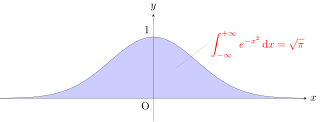
The Gaussian integral, also known as the Euler–Poisson integral, is the integral of the Gaussian function over the entire real line. Named after the German mathematician Carl Friedrich Gauss, the integral is
In mathematics, the associated Legendre polynomials are the canonical solutions of the general Legendre equation
In mathematics (specifically multivariable calculus), a multiple integral is a definite integral of a function of several real variables, for instance, f(x, y) or f(x, y, z). Physical (natural philosophy) interpretation: S any surface, V any volume, etc.. Incl. variable to time, position, etc.
A pendulum is a body suspended from a fixed support so that it swings freely back and forth under the influence of gravity. When a pendulum is displaced sideways from its resting, equilibrium position, it is subject to a restoring force due to gravity that will accelerate it back towards the equilibrium position. When released, the restoring force acting on the pendulum's mass causes it to oscillate about the equilibrium position, swinging it back and forth. The mathematics of pendulums are in general quite complicated. Simplifying assumptions can be made, which in the case of a simple pendulum allow the equations of motion to be solved analytically for small-angle oscillations.
Clenshaw–Curtis quadrature and Fejér quadrature are methods for numerical integration, or "quadrature", that are based on an expansion of the integrand in terms of Chebyshev polynomials. Equivalently, they employ a change of variables and use a discrete cosine transform (DCT) approximation for the cosine series. Besides having fast-converging accuracy comparable to Gaussian quadrature rules, Clenshaw–Curtis quadrature naturally leads to nested quadrature rules, which is important for both adaptive quadrature and multidimensional quadrature (cubature).
In mathematics, the secondary measure associated with a measure of positive density ρ when there is one, is a measure of positive density μ, turning the secondary polynomials associated with the orthogonal polynomials for ρ into an orthogonal system.
In physics and mathematics, the solid harmonics are solutions of the Laplace equation in spherical polar coordinates, assumed to be (smooth) functions . There are two kinds: the regular solid harmonics, which are well-defined at the origin and the irregular solid harmonics, which are singular at the origin. Both sets of functions play an important role in potential theory, and are obtained by rescaling spherical harmonics appropriately:
In mathematics, vector spherical harmonics (VSH) are an extension of the scalar spherical harmonics for use with vector fields. The components of the VSH are complex-valued functions expressed in the spherical coordinate basis vectors.
In the mathematical study of rotational symmetry, the zonal spherical harmonics are special spherical harmonics that are invariant under the rotation through a particular fixed axis. The zonal spherical functions are a broad extension of the notion of zonal spherical harmonics to allow for a more general symmetry group.
In mathematics, discrete Chebyshev polynomials, or Gram polynomials, are a type of discrete orthogonal polynomials used in approximation theory, introduced by Pafnuty Chebyshev and rediscovered by Gram. They were later found to be applicable to various algebraic properties of spin angular momentum.
In mathematics, Jacobi polynomials are a class of classical orthogonal polynomials. They are orthogonal with respect to the weight on the interval . The Gegenbauer polynomials, and thus also the Legendre, Zernike and Chebyshev polynomials, are special cases of the Jacobi polynomials.
Partial-wave analysis, in the context of quantum mechanics, refers to a technique for solving scattering problems by decomposing each wave into its constituent angular-momentum components and solving using boundary conditions.
This page is based on this Wikipedia article Text is available under the CC BY-SA 4.0 license; additional terms may apply. Images, videos and audio are available under their respective licenses.