Geometric transformation that preserves lines but not angles nor the origin
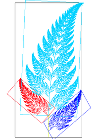
An image of a fern-like fractal (Barnsley's fern) that exhibits affine self-similarity. Each of the leaves of the fern is related to each other leaf by an affine transformation. For instance, the red leaf can be transformed into both the dark blue leaf and any of the light blue leaves by a combination of reflection, rotation, scaling, and translation.
More generally, an affine transformation is an automorphism of an affine space (Euclidean spaces are specific affine spaces), that is, a function which maps an affine space onto itself while preserving both the dimension of any affine subspaces (meaning that it sends points to points, lines to lines, planes to planes, and so on) and the ratios of the lengths of parallel line segments. Consequently, sets of parallel affine subspaces remain parallel after an affine transformation. An affine transformation does not necessarily preserve angles between lines or distances between points, though it does preserve ratios of distances between points lying on a straight line.
If X is the point set of an affine space, then every affine transformation on X can be represented as the composition of a linear transformation on X and a translation of X. Unlike a purely linear transformation, an affine transformation need not preserve the origin of the affine space. Thus, every linear transformation is affine, but not every affine transformation is linear.
A generalization of an affine transformation is an affine map[1] (or affine homomorphism or affine mapping) between two (potentially different) affine spaces over the same fieldk. Let (X, V, k) and (Z, W, k) be two affine spaces with X and Z the point sets and V and W the respective associated vector spaces over the field k. A map f: X → Z is an affine map if there exists a linear mapmf: V → W such that mf (x − y) = f (x) − f (y) for all x, y in X.[2]
Definition
Let X be an affine space over a fieldk, and V be its associated vector space. An affine transformation is a bijectionf from X onto itself that is an affine map; this means that a linear mapg from V to V is well defined by the equation here, as usual, the subtraction of two points denotes the free vector from the second point to the first one, and "well-defined" means that implies that
If the dimension of X is at least two, a semiaffine transformationf of X is a bijection from X onto itself satisfying:[3]
For every d-dimensional affine subspaceS of X, then f (S) is also a d-dimensional affine subspace of X.
If S and T are parallel affine subspaces of X, then f (S) and f (T) are parallel.
These two conditions are satisfied by affine transformations, and express what is precisely meant by the expression that "f preserves parallelism".
These conditions are not independent as the second follows from the first.[4] Furthermore, if the field k has at least three elements, the first condition can be simplified to: f is a collineation, that is, it maps lines to lines.[5]
Structure
By the definition of an affine space, V acts on X, so that, for every pair in X × V there is associated a point y in X. We can denote this action by . Here we use the convention that are two interchangeable notations for an element of V. By fixing a point c in X one can define a function mc: X → V by mc(x) = cx→. For any c, this function is one-to-one, and so, has an inverse function mc−1: V → X given by . These functions can be used to turn X into a vector space (with respect to the point c) by defining:[6]
and
This vector space has origin c and formally needs to be distinguished from the affine space X, but common practice is to denote it by the same symbol and mention that it is a vector space after an origin has been specified. This identification permits points to be viewed as vectors and vice versa.
Then L(c, λ) is an affine transformation of X which leaves the point c fixed.[7] It is a linear transformation of X, viewed as a vector space with origin c.
Let σ be any affine transformation of X. Pick a point c in X and consider the translation of X by the vector , denoted by Tw. Translations are affine transformations and the composition of affine transformations is an affine transformation. For this choice of c, there exists a unique linear transformation λ of V such that[8]
That is, an arbitrary affine transformation of X is the composition of a linear transformation of X (viewed as a vector space) and a translation of X.
This representation of affine transformations is often taken as the definition of an affine transformation (with the choice of origin being implicit).[9][10][11]
Representation
As shown above, an affine map is the composition of two functions: a translation and a linear map. Ordinary vector algebra uses matrix multiplication to represent linear maps, and vector addition to represent translations. Formally, in the finite-dimensional case, if the linear map is represented as a multiplication by an invertible matrix and the translation as the addition of a vector , an affine map acting on a vector can be represented as
Augmented matrix
Affine transformations on the 2D plane can be performed by linear transformations in three dimensions. Translation is done by shearing along over the z axis, and rotation is performed around the z axis.
Using an augmented matrix and an augmented vector, it is possible to represent both the translation and the linear map using a single matrix multiplication. The technique requires that all vectors be augmented with a "1" at the end, and all matrices be augmented with an extra row of zeros at the bottom, an extra column—the translation vector—to the right, and a "1" in the lower right corner. If is a matrix,
is equivalent to the following
The above-mentioned augmented matrix is called an affine transformation matrix. In the general case, when the last row vector is not restricted to be , the matrix becomes a projective transformation matrix (as it can also be used to perform projective transformations).
This representation exhibits the set of all invertible affine transformations as the semidirect product of and . This is a group under the operation of composition of functions, called the affine group.
Ordinary matrix-vector multiplication always maps the origin to the origin, and could therefore never represent a translation, in which the origin must necessarily be mapped to some other point. By appending the additional coordinate "1" to every vector, one essentially considers the space to be mapped as a subset of a space with an additional dimension. In that space, the original space occupies the subset in which the additional coordinate is 1. Thus the origin of the original space can be found at . A translation within the original space by means of a linear transformation of the higher-dimensional space is then possible (specifically, a shear transformation). The coordinates in the higher-dimensional space are an example of homogeneous coordinates. If the original space is Euclidean, the higher dimensional space is a real projective space.
The advantage of using homogeneous coordinates is that one can combine any number of affine transformations into one by multiplying the respective matrices. This property is used extensively in computer graphics, computer vision and robotics.
Example augmented matrix
Suppose you have three points that define a non-degenerate triangle in a plane, or four points that define a non-degenerate tetrahedron in 3-dimensional space, or generally n + 1 points x1, ..., xn+1 that define a non-degenerate simplex in n-dimensional space. Suppose you have corresponding destination points y1, ..., yn+1, where these new points can lie in a space with any number of dimensions. (Furthermore, the new points need not be distinct from each other and need not form a non-degenerate simplex.) The unique augmented matrix M that achieves the affine transformation
is
Properties
Properties preserved
An affine transformation preserves:
collinearity between points: three or more points which lie on the same line (called collinear points) continue to be collinear after the transformation.
parallelism: two or more lines which are parallel, continue to be parallel after the transformation.
convexity of sets: a convex set continues to be convex after the transformation. Moreover, the extreme points of the original set are mapped to the extreme points of the transformed set.[12]
ratios of lengths of parallel line segments: for distinct parallel segments defined by points and , and , the ratio of and is the same as that of and .
The invertible affine transformations (of an affine space onto itself) form the affine group, which has the general linear group of degree as subgroup and is itself a subgroup of the general linear group of degree .
The similarity transformations form the subgroup where is a scalar times an orthogonal matrix. For example, if the affine transformation acts on the plane and if the determinant of is 1 or −1 then the transformation is an equiareal mapping. Such transformations form a subgroup called the equi-affine group.[13] A transformation that is both equi-affine and a similarity is an isometry of the plane taken with Euclidean distance.
Each of these groups has a subgroup of orientation-preserving or positive affine transformations: those where the determinant of is positive. In the last case this is in 3D the group of rigid transformations (proper rotations and pure translations).
If there is a fixed point, we can take that as the origin, and the affine transformation reduces to a linear transformation. This may make it easier to classify and understand the transformation. For example, describing a transformation as a rotation by a certain angle with respect to a certain axis may give a clearer idea of the overall behavior of the transformation than describing it as a combination of a translation and a rotation. However, this depends on application and context.
Affine maps
An affine map between two affine spaces is a map on the points that acts linearly on the vectors (that is, the vectors between points of the space). In symbols, determines a linear transformation such that, for any pair of points :
or
.
We can interpret this definition in a few other ways, as follows.
If an origin is chosen, and denotes its image , then this means that for any vector :
.
If an origin is also chosen, this can be decomposed as an affine transformation that sends , namely
,
followed by the translation by a vector .
The conclusion is that, intuitively, consists of a translation and a linear map.
Alternative definition
Given two affine spaces and , over the same field, a function is an affine map if and only if for every family of weighted points in such that
In their applications to digital image processing, the affine transformations are analogous to printing on a sheet of rubber and stretching the sheet's edges parallel to the plane. This transform relocates pixels requiring intensity interpolation to approximate the value of moved pixels, bicubic interpolation is the standard for image transformations in image processing applications. Affine transformations scale, rotate, translate, mirror and shear images as shown in the following examples:[16]
The affine transforms are applicable to the registration process where two or more images are aligned (registered). An example of image registration is the generation of panoramic images that are the product of multiple images stitched together.
Affine warping
The affine transform preserves parallel lines. However, the stretching and shearing transformations warp shapes, as the following example shows:
This is an example of image warping. However, the affine transformations do not facilitate projection onto a curved surface or radial distortions.
In the plane
A central dilation. The triangles A1B1Z, A1C1Z, and B1C1Z get mapped to A2B2Z, A2C2Z, and B2C2Z, respectively.
Affine transformations in two real dimensions include:
pure translations,
scaling in a given direction, with respect to a line in another direction (not necessarily perpendicular), combined with translation that is not purely in the direction of scaling; taking "scaling" in a generalized sense it includes the cases that the scale factor is zero (projection) or negative; the latter includes reflection, and combined with translation it includes glide reflection,
shear mapping combined with a homothety and a translation, or
squeeze mapping combined with a homothety and a translation.
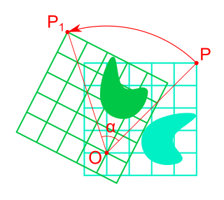
To visualise the general affine transformation of the Euclidean plane, take labelled parallelogramsABCD and A′B′C′D′. Whatever the choices of points, there is an affine transformation T of the plane taking A to A′, and each vertex similarly. Supposing we exclude the degenerate case where ABCD has zero area, there is a unique such affine transformation T. Drawing out a whole grid of parallelograms based on ABCD, the image T(P) of any point P is determined by noting that T(A) = A′, T applied to the line segment AB is A′B′, T applied to the line segment AC is A′C′, and T respects scalar multiples of vectors based at A. [If A, E, F are collinear then the ratio length(AF)/length(AE) is equal to length(A′F′)/length(A′E′).] Geometrically T transforms the grid based on ABCD to that based in A′B′C′D′.
Affine transformations do not respect lengths or angles; they multiply area by a constant factor
area of A′B′C′D′ / area of ABCD.
A given T may either be direct (respect orientation), or indirect (reverse orientation), and this may be determined by its effect on signed areas (as defined, for example, by the cross product of vectors).
Examples
Over the real numbers
The functions with and in and , are precisely the affine transformations of the real line.
In plane geometry
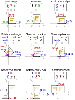
A simple affine transformation on the real planeEffect of applying various 2D affine transformation matrices on a unit square. Note that the reflection matrices are special cases of the scaling matrix.
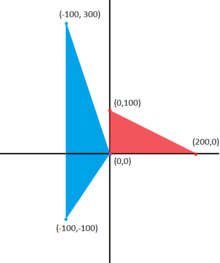
In , the transformation shown at left is accomplished using the map given by:
Transforming the three corner points of the original triangle (in red) gives three new points which form the new triangle (in blue). This transformation skews and translates the original triangle.
In fact, all triangles are related to one another by affine transformations. This is also true for all parallelograms, but not for all quadrilaterals.
See also
Anamorphosis – artistic applications of affine transformations
Euclidean space is the fundamental space of geometry, intended to represent physical space. Originally, in Euclid's Elements, it was the three-dimensional space of Euclidean geometry, but in modern mathematics there are Euclidean spaces of any positive integer dimension n, which are called Euclidean n-spaces when one wants to specify their dimension. For n equal to one or two, they are commonly called respectively Euclidean lines and Euclidean planes. The qualifier "Euclidean" is used to distinguish Euclidean spaces from other spaces that were later considered in physics and modern mathematics.
In mathematics, and more specifically in linear algebra, a linear map is a mapping between two vector spaces that preserves the operations of vector addition and scalar multiplication. The same names and the same definition are also used for the more general case of modules over a ring; see Module homomorphism.
In physics, the Lorentz transformations are a six-parameter family of linear transformations from a coordinate frame in spacetime to another frame that moves at a constant velocity relative to the former. The respective inverse transformation is then parameterized by the negative of this velocity. The transformations are named after the Dutch physicist Hendrik Lorentz.
In mathematical physics and mathematics, the Pauli matrices are a set of three 2 × 2 complex matrices that are Hermitian, involutory and unitary. Usually indicated by the Greek letter sigma, they are occasionally denoted by tau when used in connection with isospin symmetries.
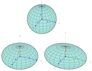
An ellipsoid is a surface that can be obtained from a sphere by deforming it by means of directional scalings, or more generally, of an affine transformation.
In mathematics, a quadric or quadric surface (quadric hypersurface in higher dimensions), is a generalization of conic sections (ellipses, parabolas, and hyperbolas). It is a hypersurface (of dimension D) in a (D + 1)-dimensional space, and it is defined as the zero set of an irreducible polynomial of degree two in D + 1 variables; for example, D = 1 in the case of conic sections. When the defining polynomial is not absolutely irreducible, the zero set is generally not considered a quadric, although it is often called a degenerate quadric or a reducible quadric.
In the mathematical field of differential geometry, a metric tensor is an additional structure on a manifold M that allows defining distances and angles, just as the inner product on a Euclidean space allows defining distances and angles there. More precisely, a metric tensor at a point p of M is a bilinear form defined on the tangent space at p, and a metric field on M consists of a metric tensor at each point p of M that varies smoothly with p.
In Euclidean geometry, a translation is a geometric transformation that moves every point of a figure, shape or space by the same distance in a given direction. A translation can also be interpreted as the addition of a constant vector to every point, or as shifting the origin of the coordinate system. In a Euclidean space, any translation is an isometry.
In physics and mathematics, the Lorentz group is the group of all Lorentz transformations of Minkowski spacetime, the classical and quantum setting for all (non-gravitational) physical phenomena. The Lorentz group is named for the Dutch physicist Hendrik Lorentz.
In mathematics, the affine group or general affine group of any affine space is the group of all invertible affine transformations from the space into itself. In the case of a Euclidean space, the affine group consists of those functions from the space to itself such that the image of every line is a line.
In mathematics, an affine space is a geometric structure that generalizes some of the properties of Euclidean spaces in such a way that these are independent of the concepts of distance and measure of angles, keeping only the properties related to parallelism and ratio of lengths for parallel line segments. Affine space is the setting for affine geometry.
Rotation in mathematics is a concept originating in geometry. Any rotation is a motion of a certain space that preserves at least one point. It can describe, for example, the motion of a rigid body around a fixed point. Rotation can have a sign (as in the sign of an angle): a clockwise rotation is a negative magnitude so a counterclockwise turn has a positive magnitude. A rotation is different from other types of motions: translations, which have no fixed points, and (hyperplane) reflections, each of them having an entire (n − 1)-dimensional flat of fixed points in a n-dimensional space.
In mathematics, an invariant subspace of a linear mapping T : V → V i.e. from some vector space V to itself, is a subspace W of V that is preserved by T. More generally, an invariant subspace for a collection of linear mappings is a subspace preserved by each mapping individually.
In linear algebra, linear transformations can be represented by matrices. If is a linear transformation mapping to and is a column vector with entries, then
In mathematics, the Kronecker product, sometimes denoted by ⊗, is an operation on two matrices of arbitrary size resulting in a block matrix. It is a specialization of the tensor product from vectors to matrices and gives the matrix of the tensor product linear map with respect to a standard choice of basis. The Kronecker product is to be distinguished from the usual matrix multiplication, which is an entirely different operation. The Kronecker product is also sometimes called matrix direct product.
In geometry, a barycentric coordinate system is a coordinate system in which the location of a point is specified by reference to a simplex. The barycentric coordinates of a point can be interpreted as masses placed at the vertices of the simplex, such that the point is the center of mass of these masses. These masses can be zero or negative; they are all positive if and only if the point is inside the simplex.
Screw theory is the algebraic calculation of pairs of vectors, such as angular and linear velocity, or forces and moments, that arise in the kinematics and dynamics of rigid bodies.
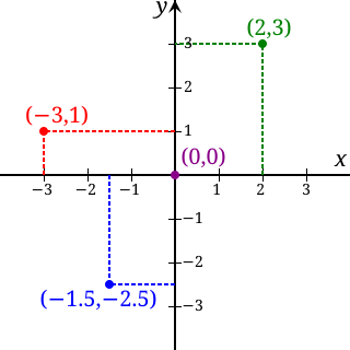
In mathematics, the real coordinate space or real coordinate n-space, of dimension n, denoted Rn or , is the set of all ordered n-tuples of real numbers, that is the set of all sequences of n real numbers, also known as coordinate vectors. Special cases are called the real lineR1, the real coordinate planeR2, and the real coordinate three-dimensional spaceR3. With component-wise addition and scalar multiplication, it is a real vector space.
In geometry, a set of points in space are coplanar if there exists a geometric plane that contains them all. For example, three points are always coplanar, and if the points are distinct and non-collinear, the plane they determine is unique. However, a set of four or more distinct points will, in general, not lie in a single plane.
This page is based on this Wikipedia article Text is available under the CC BY-SA 4.0 license; additional terms may apply. Images, videos and audio are available under their respective licenses.