
In mathematics, the Lyapunov exponent or Lyapunov characteristic exponent of a dynamical system is a quantity that characterizes the rate of separation of infinitesimally close trajectories. Quantitatively, two trajectories in phase space with initial separation vector diverge at a rate given by
In quantum mechanics, perturbation theory is a set of approximation schemes directly related to mathematical perturbation for describing a complicated quantum system in terms of a simpler one. The idea is to start with a simple system for which a mathematical solution is known, and add an additional "perturbing" Hamiltonian representing a weak disturbance to the system. If the disturbance is not too large, the various physical quantities associated with the perturbed system can be expressed as "corrections" to those of the simple system. These corrections, being small compared to the size of the quantities themselves, can be calculated using approximate methods such as asymptotic series. The complicated system can therefore be studied based on knowledge of the simpler one. In effect, it is describing a complicated unsolved system using a simple, solvable system.
In mathematics, the Rayleigh quotient for a given complex Hermitian matrix and nonzero vector is defined as:

Various types of stability may be discussed for the solutions of differential equations or difference equations describing dynamical systems. The most important type is that concerning the stability of solutions near to a point of equilibrium. This may be discussed by the theory of Aleksandr Lyapunov. In simple terms, if the solutions that start out near an equilibrium point stay near forever, then is Lyapunov stable. More strongly, if is Lyapunov stable and all solutions that start out near converge to , then is said to be asymptotically stable. The notion of exponential stability guarantees a minimal rate of decay, i.e., an estimate of how quickly the solutions converge. The idea of Lyapunov stability can be extended to infinite-dimensional manifolds, where it is known as structural stability, which concerns the behavior of different but "nearby" solutions to differential equations. Input-to-state stability (ISS) applies Lyapunov notions to systems with inputs.
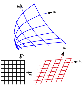
In geometry, curvilinear coordinates are a coordinate system for Euclidean space in which the coordinate lines may be curved. These coordinates may be derived from a set of Cartesian coordinates by using a transformation that is locally invertible at each point. This means that one can convert a point given in a Cartesian coordinate system to its curvilinear coordinates and back. The name curvilinear coordinates, coined by the French mathematician Lamé, derives from the fact that the coordinate surfaces of the curvilinear systems are curved.
In electrical engineering, a differential-algebraic system of equations (DAEs) is a system of equations that either contains differential equations and algebraic equations, or is equivalent to such a system. In mathematics these are examples of differential algebraic varieties and correspond to ideals in differential polynomial rings (see the article on differential algebra for the algebraic setup.
In linear algebra, an eigenvector or characteristic vector of a linear transformation is a nonzero vector that changes at most by a scalar factor when that linear transformation is applied to it. The corresponding eigenvalue, often denoted by , is the factor by which the eigenvector is scaled.
The Lanczos algorithm is an iterative method devised by Cornelius Lanczos that is an adaptation of power methods to find the "most useful" eigenvalues and eigenvectors of an Hermitian matrix, where is often but not necessarily much smaller than . Although computationally efficient in principle, the method as initially formulated was not useful, due to its numerical instability.

In the study of dynamical systems, a hyperbolic equilibrium point or hyperbolic fixed point is a fixed point that does not have any center manifolds. Near a hyperbolic point the orbits of a two-dimensional, non-dissipative system resemble hyperbolas. This fails to hold in general. Strogatz notes that "hyperbolic is an unfortunate name—it sounds like it should mean 'saddle point'—but it has become standard." Several properties hold about a neighborhood of a hyperbolic point, notably
In mathematics, preconditioning is the application of a transformation, called the preconditioner, that conditions a given problem into a form that is more suitable for numerical solving methods. Preconditioning is typically related to reducing a condition number of the problem. The preconditioned problem is then usually solved by an iterative method.

In mathematics, stability theory addresses the stability of solutions of differential equations and of trajectories of dynamical systems under small perturbations of initial conditions. The heat equation, for example, is a stable partial differential equation because small perturbations of initial data lead to small variations in temperature at a later time as a result of the maximum principle. In partial differential equations one may measure the distances between functions using Lp norms or the sup norm, while in differential geometry one may measure the distance between spaces using the Gromov–Hausdorff distance.
In theoretical physics, the BRST formalism, or BRST quantization denotes a relatively rigorous mathematical approach to quantizing a field theory with a gauge symmetry. Quantization rules in earlier quantum field theory (QFT) frameworks resembled "prescriptions" or "heuristics" more than proofs, especially in non-abelian QFT, where the use of "ghost fields" with superficially bizarre properties is almost unavoidable for technical reasons related to renormalization and anomaly cancellation.
In computational chemistry, a constraint algorithm is a method for satisfying the Newtonian motion of a rigid body which consists of mass points. A restraint algorithm is used to ensure that the distance between mass points is maintained. The general steps involved are: (i) choose novel unconstrained coordinates, (ii) introduce explicit constraint forces, (iii) minimize constraint forces implicitly by the technique of Lagrange multipliers or projection methods.
Numerical continuation is a method of computing approximate solutions of a system of parameterized nonlinear equations,
Synchronization of chaos is a phenomenon that may occur when two or more dissipative chaotic systems are coupled.
In linear algebra, eigendecomposition is the factorization of a matrix into a canonical form, whereby the matrix is represented in terms of its eigenvalues and eigenvectors. Only diagonalizable matrices can be factorized in this way. When the matrix being factorized is a normal or real symmetric matrix, the decomposition is called "spectral decomposition", derived from the spectral theorem.
Non-linear least squares is the form of least squares analysis used to fit a set of m observations with a model that is non-linear in n unknown parameters (m ≥ n). It is used in some forms of nonlinear regression. The basis of the method is to approximate the model by a linear one and to refine the parameters by successive iterations. There are many similarities to linear least squares, but also some significant differences. In economic theory, the non-linear least squares method is applied in (i) the probit regression, (ii) threshold regression, (iii) smooth regression, (iv) logistic link regression, (v) Box–Cox transformed regressors ().

Lagrangian coherent structures (LCSs) are distinguished surfaces of trajectories in a dynamical system that exert a major influence on nearby trajectories over a time interval of interest. The type of this influence may vary, but it invariably creates a coherent trajectory pattern for which the underlying LCS serves as a theoretical centerpiece. In observations of tracer patterns in nature, one readily identifies coherent features, but it is often the underlying structure creating these features that is of interest.

In chaos theory and fluid dynamics, chaotic mixing is a process by which flow tracers develop into complex fractals under the action of a fluid flow. The flow is characterized by an exponential growth of fluid filaments. Even very simple flows, such as the blinking vortex, or finitely resolved wind fields can generate exceptionally complex patterns from initially simple tracer fields.
In the mathematics of dynamical systems, the concept of Lyapunov dimension was suggested by Kaplan and Yorke for estimating the Hausdorff dimension of attractors. Further the concept has been developed and rigorously justified in a number of papers, and nowadays various different approaches to the definition of Lyapunov dimension are used. Remark that the attractors with noninteger Hausdorff dimension are called strange attractors. Since the direct numerical computation of the Hausdorff dimension of attractors is often a problem of high numerical complexity, estimations via the Lyapunov dimension became widely spread. The Lyapunov dimension was named after the Russian mathematician Aleksandr Lyapunov because of the close connection with the Lyapunov exponents.


