Model order reduction

Last updated

Model order reduction (MOR) is a technique for reducing the computational complexity of mathematical models in numerical simulations. As such it is closely related to the concept of metamodeling, with applications in all areas of mathematical modelling.

Contents

Overview

Many modern mathematical models of real-life processes pose challenges when used in numerical simulations, due to complexity and large size (dimension). Model order reduction aims to lower the computational complexity of such problems, for example, in simulations of large-scale dynamical systems and control systems. By a reduction of the model's associated state space dimension or degrees of freedom, an approximation to the original model is computed which is commonly referred to as a reduced order model.

Reduced order models are useful in settings where it is often unfeasible to perform numerical simulations using the complete full order model. This can be due to limitations in computational resources or the requirements of the simulations setting, for instance real-time simulation settings or many-query settings in which a large number of simulations needs to be performed. [1] [2] Examples of Real-time simulation settings include control systems in electronics and visualization of model results while examples for a many-query setting can include optimization problems and design exploration. In order to be applicable to real-world problems, often the requirements of a reduced order model are: [3] [4]

It is interesting to note that in some cases (e.g. constrained lumping of polynomial differential equations) it is possible to have a null approximation error, resulting in an exact model order reduction. [5]

Methods

Contemporary model order reduction techniques can be broadly classified into 5 classes: [1] [6]

The simplified physics approach can be described to be analogous to the traditional mathematical modelling approach, in which a less complex description of a system is constructed based on assumptions and simplifications using physical insight or otherwise derived information. However, this approach is not often the topic of discussion in the context of model order reduction as it is a general method in science, engineering, and mathematics.

The remaining listed methods fall into the category of projection-based reduction. Projection-based reduction relies on the projection of either the model equations or the solution onto a basis of reduced dimensionality compared to the original solution space. Methods that also fall into this class but are perhaps less common are:

Implementations

Applications

Model order reduction finds application within all fields involving mathematical modelling and many reviews [10] [13] exist for the topics of electronics, [17] fluid mechanics, [18] hydrodynamics, [16] structural mechanics, [7] MEMS, [19] Boltzmann equation, [8] and design optimization. [14] [20]

Fluid mechanics

Current problems in fluid mechanics involve large dynamical systems representing many effects on many different scales. Computational fluid dynamics studies often involve models solving the Navier–Stokes equations with a number of degrees of freedom in the order of magnitude upwards of . The first usage of model order reduction techniques dates back to the work of Lumley in 1967, [21] where it was used to gain insight into the mechanisms and intensity of turbulence and large coherent structures present in fluid flow problems. Model order reduction also finds modern applications in aeronautics to model the flow over the body of aircraft. [22] An example can be found in Lieu et al [23] in which the full order model of an F16 fighter-aircraft with over 2.1 million degrees of freedom, was reduced to a model of just 90 degrees of freedom. Additionally reduced order modeling has been applied to study rheology in hemodynamics and the fluid–structure interaction between the blood flowing through the vascular system and the vascular walls. [24] [25]

See also

Related Research Articles

<span class="mw-page-title-main">Computational chemistry</span> Branch of chemistry

Computational chemistry is a branch of chemistry that uses computer simulations to assist in solving chemical problems. It uses methods of theoretical chemistry incorporated into computer programs to calculate the structures and properties of molecules, groups of molecules, and solids. The importance of this subject stems from the fact that, with the exception of some relatively recent findings related to the hydrogen molecular ion, achieving an accurate quantum mechanical depiction of chemical systems analytically, or in a closed form, is not feasible. The complexity inherent in the many-body problem exacerbates the challenge of providing detailed descriptions of quantum mechanical systems. While computational results normally complement information obtained by chemical experiments, it can occasionally predict unobserved chemical phenomena.

Monte Carlo methods, or Monte Carlo experiments, are a broad class of computational algorithms that rely on repeated random sampling to obtain numerical results. The underlying concept is to use randomness to solve problems that might be deterministic in principle. The name comes from the Monte Carlo Casino in Monaco, where the primary developer of the method, physicist Stanislaw Ulam, was inspired by his uncle's gambling habits.

<span class="mw-page-title-main">Computational physics</span> Numerical simulations of physical problems via computers

Computational physics is the study and implementation of numerical analysis to solve problems in physics. Historically, computational physics was the first application of modern computers in science, and is now a subset of computational science. It is sometimes regarded as a subdiscipline of theoretical physics, but others consider it an intermediate branch between theoretical and experimental physics — an area of study which supplements both theory and experiment.

In mathematics and science, a nonlinear system is a system in which the change of the output is not proportional to the change of the input. Nonlinear problems are of interest to engineers, biologists, physicists, mathematicians, and many other scientists since most systems are inherently nonlinear in nature. Nonlinear dynamical systems, describing changes in variables over time, may appear chaotic, unpredictable, or counterintuitive, contrasting with much simpler linear systems.

<span class="mw-page-title-main">Computational fluid dynamics</span> Analysis and solving of problems that involve fluid flows

Computational fluid dynamics (CFD) is a branch of fluid mechanics that uses numerical analysis and data structures to analyze and solve problems that involve fluid flows. Computers are used to perform the calculations required to simulate the free-stream flow of the fluid, and the interaction of the fluid with surfaces defined by boundary conditions. With high-speed supercomputers, better solutions can be achieved, and are often required to solve the largest and most complex problems. Ongoing research yields software that improves the accuracy and speed of complex simulation scenarios such as transonic or turbulent flows. Initial validation of such software is typically performed using experimental apparatus such as wind tunnels. In addition, previously performed analytical or empirical analysis of a particular problem can be used for comparison. A final validation is often performed using full-scale testing, such as flight tests.

<span class="mw-page-title-main">System identification</span> Statistical methods to build mathematical models of dynamical systems from measured data

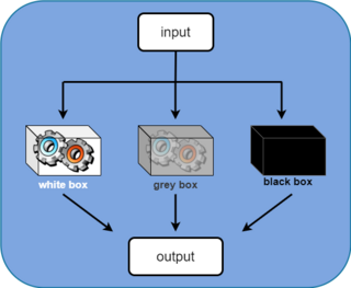
The field of system identification uses statistical methods to build mathematical models of dynamical systems from measured data. System identification also includes the optimal design of experiments for efficiently generating informative data for fitting such models as well as model reduction. A common approach is to start from measurements of the behavior of the system and the external influences and try to determine a mathematical relation between them without going into many details of what is actually happening inside the system; this approach is called black box system identification.

Numerical methods for partial differential equations is the branch of numerical analysis that studies the numerical solution of partial differential equations (PDEs).

<span class="mw-page-title-main">Finite-difference time-domain method</span> Numerical analysis technique

Finite-difference time-domain (FDTD) or Yee's method is a numerical analysis technique used for modeling computational electrodynamics. Since it is a time-domain method, FDTD solutions can cover a wide frequency range with a single simulation run, and treat nonlinear material properties in a natural way.

<span class="mw-page-title-main">Lorenz system</span> System of ordinary differential equations with chaotic solutions

The Lorenz system is a system of ordinary differential equations first studied by mathematician and meteorologist Edward Lorenz. It is notable for having chaotic solutions for certain parameter values and initial conditions. In particular, the Lorenz attractor is a set of chaotic solutions of the Lorenz system. The term "butterfly effect" in popular media may stem from the real-world implications of the Lorenz attractor, namely that several different initial chaotic conditions evolve in phase space in a way that never repeats, so all chaos is unpredictable. This underscores that chaotic systems can be completely deterministic and yet still be inherently unpredictable over long periods of time. Because chaos continually increases in systems, we cannot predict the future of systems well. E.g., even the small flap of a butterfly’s wings could set the world on a vastly different trajectory, such as by causing a hurricane. The shape of the Lorenz attractor itself, when plotted in phase space, may also be seen to resemble a butterfly.

<span class="mw-page-title-main">Fluid–structure interaction</span>

Fluid–structure interaction (FSI) is the interaction of some movable or deformable structure with an internal or surrounding fluid flow. Fluid–structure interactions can be stable or oscillatory. In oscillatory interactions, the strain induced in the solid structure causes it to move such that the source of strain is reduced, and the structure returns to its former state only for the process to repeat.

<span class="mw-page-title-main">Meshfree methods</span> Methods in numerical analysis not requiring knowledge of neighboring points

In the field of numerical analysis, meshfree methods are those that do not require connection between nodes of the simulation domain, i.e. a mesh, but are rather based on interaction of each node with all its neighbors. As a consequence, original extensive properties such as mass or kinetic energy are no longer assigned to mesh elements but rather to the single nodes. Meshfree methods enable the simulation of some otherwise difficult types of problems, at the cost of extra computing time and programming effort. The absence of a mesh allows Lagrangian simulations, in which the nodes can move according to the velocity field.

<span class="mw-page-title-main">Finite element method</span> Numerical method for solving physical or engineering problems

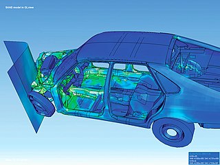
The finite element method (FEM) is a popular method for numerically solving differential equations arising in engineering and mathematical modeling. Typical problem areas of interest include the traditional fields of structural analysis, heat transfer, fluid flow, mass transport, and electromagnetic potential.

Dynamic mode decomposition (DMD) is a dimensionality reduction algorithm developed by Peter J. Schmid and Joern Sesterhenn in 2008. Given a time series of data, DMD computes a set of modes each of which is associated with a fixed oscillation frequency and decay/growth rate. For linear systems in particular, these modes and frequencies are analogous to the normal modes of the system, but more generally, they are approximations of the modes and eigenvalues of the composition operator. Due to the intrinsic temporal behaviors associated with each mode, DMD differs from dimensionality reduction methods such as principal component analysis, which computes orthogonal modes that lack predetermined temporal behaviors. Because its modes are not orthogonal, DMD-based representations can be less parsimonious than those generated by PCA. However, they can also be more physically meaningful because each mode is associated with a damped sinusoidal behavior in time.

<span class="mw-page-title-main">Homotopy analysis method</span>

The homotopy analysis method (HAM) is a semi-analytical technique to solve nonlinear ordinary/partial differential equations. The homotopy analysis method employs the concept of the homotopy from topology to generate a convergent series solution for nonlinear systems. This is enabled by utilizing a homotopy-Maclaurin series to deal with the nonlinearities in the system.

<span class="mw-page-title-main">MOOSE (software)</span>

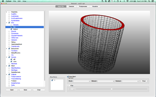
MOOSE is an object-oriented C++ finite element framework for the development of tightly coupled multiphysics solvers from Idaho National Laboratory. MOOSE makes use of the PETSc non-linear solver package and libmesh to provide the finite element discretization.

<span class="mw-page-title-main">Parareal</span> Parallel algorithm from numerical analysis

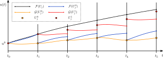
Parareal is a parallel algorithm from numerical analysis and used for the solution of initial value problems. It was introduced in 2001 by Lions, Maday and Turinici. Since then, it has become one of the most widely studied parallel-in-time integration methods.

Nektar++ is a spectral/hp element framework designed to support the construction of efficient high-performance scalable solvers for a wide range of partial differential equations (PDE). The code is released as open-source under the MIT license. Although primarily driven by application-based research, it has been designed as a platform to support the development of novel numerical techniques in the area of high-order finite element methods.

The proper generalized decomposition (PGD) is an iterative numerical method for solving boundary value problems (BVPs), that is, partial differential equations constrained by a set of boundary conditions, such as the Poisson's equation or the Laplace's equation.

<span class="mw-page-title-main">Physics-informed neural networks</span> Technique to solve partial differential equations

Physics-informed neural networks (PINNs) are a type of universal function approximators that can embed the knowledge of any physical laws that govern a given data-set in the learning process, and can be described by partial differential equations (PDEs). They overcome the low data availability of some biological and engineering systems that makes most state-of-the-art machine learning techniques lack robustness, rendering them ineffective in these scenarios. The prior knowledge of general physical laws acts in the training of neural networks (NNs) as a regularization agent that limits the space of admissible solutions, increasing the correctness of the function approximation. This way, embedding this prior information into a neural network results in enhancing the information content of the available data, facilitating the learning algorithm to capture the right solution and to generalize well even with a low amount of training examples.

References

  1. 1 2 Lassila, Toni; Manzoni, Andrea; Quarteroni, Alfio; Rozza, Gianluigi (2014). "Model Order Reduction in Fluid Dynamics: Challenges and Perspectives". Reduced Order Methods for Modeling and Computational Reduction (PDF). pp. 235–273. doi:10.1007/978-3-319-02090-7_9. ISBN   978-3-319-02089-1.
  2. Rozza, G.; Huynh, D. B. P.; Patera, A. T. (2008-05-21). "Reduced Basis Approximation and a Posteriori Error Estimation for Affinely Parametrized Elliptic Coercive Partial Differential Equations". Archives of Computational Methods in Engineering. 15 (3): 229–275. doi:10.1007/s11831-008-9019-9. ISSN   1134-3060. S2CID   13511413.
  3. 1 2 Schilders, Wilhelmus; van der Vorst, Henk; Rommes, Joost (2008). Model Order Reduction: Theory, Research Aspects and Applications. Springer-Verlag. ISBN   978-3-540-78841-6.
  4. Antoulas, A.C. (July 2004). "Approximation of Large-Scale Dynamical Systems: An Overview". IFAC Proceedings Volumes. 37 (11): 19–28. CiteSeerX   10.1.1.29.3565 . doi:10.1016/S1474-6670(17)31584-7.
  5. Ovchinnikov, Alexey; Pérez Verona, Isabel; Pogudin, Gleb; Tribastone, Mirco (2021-07-19). Valencia, Alfonso (ed.). "CLUE: exact maximal reduction of kinetic models by constrained lumping of differential equations". Bioinformatics. 37 (12): 1732–1738. arXiv: 2004.11961 . doi: 10.1093/bioinformatics/btab010 . ISSN   1367-4803. PMID   33532849.
  6. Silva, João M. S.; Villena, Jorge Fernández; Flores, Paulo; Silveira, L. Miguel (2007), "Outstanding Issues in Model Order Reduction", Scientific Computing in Electrical Engineering, Springer Berlin Heidelberg, pp. 139–152, doi:10.1007/978-3-540-71980-9_13, ISBN   978-3-540-71979-3
  7. 1 2 Kerschen, Gaetan; Golinval, Jean-claude; VAKAKIS, ALEXANDER F.; BERGMAN, LAWRENCE A. (2005). "The Method of Proper Orthogonal Decomposition for Dynamical Characterization and Order Reduction of Mechanical Systems: An Overview". Nonlinear Dynamics. 41 (1–3): 147–169. CiteSeerX   10.1.1.530.8349 . doi:10.1007/s11071-005-2803-2. ISSN   0924-090X. S2CID   17625377.
  8. 1 2 Choi, Youngsoo; Brown, Peter; Arrighi, William; Anderson, Robert; Huynh, Kevin (2021). "Space--time reduced order model for large-scale linear dynamical systems with application to Boltzmann transport problems". Journal of Computational Physics. 424: 109845. arXiv: 1910.01260 . Bibcode:2021JCoPh.42409845C. doi:10.1016/j.jcp.2020.109845. ISSN   0021-9991. S2CID   203641768.
  9. Boyaval, S.; Le Bris, C.; Lelièvre, T.; Maday, Y.; Nguyen, N. C.; Patera, A. T. (16 October 2010). "Reduced Basis Techniques for Stochastic Problems". Archives of Computational Methods in Engineering. 17 (4): 435–454. arXiv: 1004.0357 . doi:10.1007/s11831-010-9056-z. hdl:1721.1/63915. S2CID   446613.
  10. 1 2 Benner, Peter; Gugercin, Serkan; Willcox, Karen (2015). "A Survey of Projection-Based Model Reduction Methods for Parametric Dynamical Systems" (PDF). SIAM Review. 57 (4): 483–531. doi:10.1137/130932715. hdl: 1721.1/100939 . ISSN   0036-1445. S2CID   16186635.
  11. Kim, Youngkyu; Choi, Youngsoo; Widemann, David; Zohdi, Tarek (2021). "A fast and accurate physics-informed neural network reduced order model with shallow masked autoencoder". Journal of Computational Physics. 451: 110841. arXiv: 2009.11990 . doi:10.1016/j.jcp.2021.110841. S2CID   221949087.
  12. Mojgani, Rambod; Balajewicz, Maciej (2021). "Low-Rank Registration Based Manifolds for Convection-Dominated PDEs". Proceedings of the AAAI Conference on Artificial Intelligence. 35: 399-407. arXiv: 2006.15655 . doi: 10.1609/aaai.v35i1.16116 . S2CID   220249659.
  13. 1 2 Chinesta, Francisco; Ladeveze, Pierre; Cueto, Elías (11 October 2011). "A Short Review on Model Order Reduction Based on Proper Generalized Decomposition" (PDF). Archives of Computational Methods in Engineering. 18 (4): 395–404. doi:10.1007/s11831-011-9064-7. S2CID   54512292.
  14. 1 2 Choi, Youngsoo; Boncoraglio, Gabriele; Spenser, Anderson; Amsallem, David; Farhat, Charbel (2020). "Gradient-based constrained optimization using a database of linear reduced-order models". Journal of Computational Physics. 423: 109787. arXiv: 1506.07849 . Bibcode:2020JCoPh.42309787C. doi:10.1016/j.jcp.2020.109787. S2CID   60788542.
  15. Bai, Zhaojun (2002). "Krylov subspace techniques for reduced-order modeling of large-scale dynamical systems". Applied Numerical Mathematics. 43 (1–2): 9–44. CiteSeerX   10.1.1.131.8251 . doi:10.1016/S0168-9274(02)00116-2.
  16. 1 2 Copeland, Dylan; Cheung, Siu Wun; Huynh, Kevin; Choi, Youngsoo (2021). "Reduced order models for Lagrangian hydrodynamics". Computer Methods in Applied Mechanics and Engineering. 388: 114259. arXiv: 2104.11404 . doi:10.1016/j.cma.2021.114259. ISSN   0045-7825. S2CID   233388014.
  17. Umunnakwe, Chisom Bernhard; Zawra, Ibrahim; Niessner, Martin; Rudnyi, Evgenii; Hohlfeld, Dennis; Bechtold, Tamara (2023). "Compact modelling of a thermo-mechanical finite element model of a microelectronic package". Microelectronics Reliability. 151 (115238). doi:10.1016/j.microrel.2023.115238.
  18. Holmes, Philip; Lumley, John L.; Berkooz, Gal (1996). Turbulence, Coherent Structures, Dynamical Systems and Symmetry. Cambridge: Cambridge University Press. doi:10.1017/cbo9780511622700. ISBN   978-0-511-62270-0.
  19. Bechtold, Tamara; Schrag, Gabriela; Feng, Lihong (2013). System-Level Modeling of MEMS. Wiley-VCH Verlag GmbH & Co. KGaA. ISBN   978-3-527-31903-9.
  20. McBane, Sean; Choi, Youngsoo (1 August 2021). "Component-wise reduced order model lattice-type structure design". Computer Methods in Applied Mechanics and Engineering. 381 (113813): 113813. arXiv: 2010.10770 . Bibcode:2021CMAME.381k3813M. doi:10.1016/j.cma.2021.113813. S2CID   224818337.
  21. Lumley, J.L. (1967). The Structure of Inhomogeneous Turbulence," In: A. M. Yaglom and V. I. Tatarski, Eds., Atmospheric Turbulence and Wave Propagation. Moscow: Nauka.
  22. Walton, S.; Hassan, O.; Morgan, K. (2013). "Reduced order modelling for unsteady fluid flow using proper orthogonal decomposition and radial basis functions". Applied Mathematical Modelling. 37 (20–21): 8930–8945. doi: 10.1016/j.apm.2013.04.025 . ISSN   0307-904X.
  23. Lieu, T.; Farhat, C.; Lesoinne, M. (2006). "Reduced-order fluid/structure modeling of a complete aircraft configuration". Computer Methods in Applied Mechanics and Engineering. 195 (41–43): 5730–5742. Bibcode:2006CMAME.195.5730L. doi:10.1016/j.cma.2005.08.026. ISSN   0045-7825.
  24. Xiao, D.; Yang, P.; Fang, F.; Xiang, J.; Pain, C.C.; Navon, I.M. (2016). "Non-intrusive reduced order modelling of fluid–structure interactions" (PDF). Computer Methods in Applied Mechanics and Engineering. 303: 35–54. Bibcode:2016CMAME.303...35X. doi: 10.1016/j.cma.2015.12.029 . ISSN   0045-7825.
  25. Colciago, C.M.; Deparis, S.; Quarteroni, A. (2014). "Comparisons between reduced order models and full 3D models for fluid–structure interaction problems in haemodynamics". Journal of Computational and Applied Mathematics. 265: 120–138. doi: 10.1016/j.cam.2013.09.049 . ISSN   0377-0427.

Further reading