Parameters characterizing properties of our galaxy
The Oort constants (discovered by Jan Oort) and are empirically derived parameters that characterize the local rotational properties of our galaxy, the Milky Way, in the following manner:
where and are the rotational velocity and distance to the Galactic Center, respectively, measured at the position of the Sun, and v and r are the velocities and distances at other positions in our part of the galaxy. As derived below, A and B depend only on the motions and positions of stars in the solar neighborhood. As of 2018, the most accurate values of these constants are = 15.3 ± 0.4 km s−1 kpc−1, = −11.9 ± 0.4 km s−1 kpc−1.[1] From the Oort constants, it is possible to determine the orbital properties of the Sun, such as the orbital velocity and period, and infer local properties of the Galactic disk, such as the mass density and how the rotational velocity changes as a function of radius from the Galactic Center.
Historical significance and background
Orbits of stars around the galactic disk with faster angular velocity closer to the Galaxy Center but colored as seen from the Sun and plotted against the galactic longitude together with the same graph using data from Gaia
By the 1920s, a large fraction of the astronomical community had recognized that some of the diffuse, cloud-like objects, or nebulae, seen in the night sky were collections of stars located beyond our own, local collection of star clusters. These galaxies had diverse morphologies, ranging from ellipsoids to disks. The concentrated band of starlight that is the visible signature of the Milky Way was indicative of a disk structure for our galaxy; however, our location within our galaxy made structural determinations from observations difficult.
Classical mechanics predicted that a collection of stars could be supported against gravitational collapse by either random velocities of the stars or their rotation about its center of mass.[4] For a disk-shaped collection, the support should be mainly rotational. Depending on the mass density, or distribution of the mass in the disk, the rotation velocity may be different at each radius from the center of the disk to the outer edge. A plot of these rotational velocities against the radii at which they are measured is called a rotation curve. For external disk galaxies, one can measure the rotation curve by observing the Doppler shifts of spectral features measured along different galactic radii, since one side of the galaxy will be moving towards our line of sight and one side away. However, our position in the Galactic midplane of the Milky Way, where dust in molecular clouds obscures most optical light in many directions, made obtaining our own rotation curve technically difficult until the discovery of the 21 cm hydrogen line in the 1930s.
To confirm the rotation of our galaxy prior to this, in 1927 Jan Oort derived a way to measure the Galactic rotation from just a small fraction of stars in the local neighborhood.[5] As described below, the values he found for and proved not only that the Galaxy was rotating but also that it rotates differentially, or as a fluid rather than a solid body.
Derivation
Figure 1: Geometry of the Oort constants derivation, with a field star close to the Sun in the midplane of the Galaxy.
Consider a star in the midplane of the Galactic disk with Galactic longitude at a distance from the Sun. Assume that both the star and the Sun have circular orbits around the center of the Galaxy at radii of and from the Galactic Center and rotational velocities of and , respectively. The motion of the star along our line of sight, or radial velocity, and motion of the star across the plane of the sky, or transverse velocity, as observed from the position of the Sun are then:
With the assumption of circular motion, the rotational velocity is related to the angular velocity by and we can substitute this into the velocity expressions:
From the geometry in Figure 1, one can see that the triangles formed between the Galactic Center, the Sun, and the star share a side or portions of sides, so the following relationships hold and substitutions can be made:
and with these we get
To put these expressions only in terms of the known quantities and , we take a Taylor expansion of about .
Additionally, we take advantage of the assumption that the stars used for this analysis are local, i.e. is small, and the distance d to the star is smaller than or , and we take:
Using the sine and cosine half angle formulae, these velocities may be rewritten as:
Writing the velocities in terms of our known quantities and two coefficients and yields:
where
At this stage, the observable velocities are related to these coefficients and the position of the star. It is now possible to relate these coefficients to the rotation properties of the galaxy. For a star in a circular orbit, we can express the derivative of the angular velocity with respect to radius in terms of the rotation velocity and radius and evaluate this at the location of the Sun:
so
Oort constants on a wall in Leiden
is the Oort constant describing the shearing motion and is the Oort constant describing the rotation of the Galaxy. As described below, one can measure and from plotting these velocities, measured for many stars, against the galactic longitudes of these stars.
Measurements
Figure 2: Measuring the Oort constants by fitting to large data sets. Note that this graph erroneously shows B as positive. A negative B value contributes a westerly component to the transverse velocities.
As mentioned in an intermediate step in the derivation above:
Therefore, we can write the Oort constants and as:
Thus, the Oort constants can be expressed in terms of the radial and transverse velocities, distances, and galactic longitudes of objects in our Galaxy - all of which are, in principle, observable quantities.
However, there are a number of complications. The simple derivation above assumed that both the Sun and the object in question are traveling on circular orbits about the Galactic center. This is not true for the Sun (the Sun's velocity relative to the local standard of rest is approximately 13.4km/s),[6] and not necessarily true for other objects in the Milky Way either. The derivation also implicitly assumes that the gravitational potential of the Milky Way is axisymmetric and always directed towards the center. This ignores the effects of spiral arms and the Galaxy's bar. Finally, both transverse velocity and distance are notoriously difficult to measure for objects which are not relatively nearby.
Since the non-circular component of the Sun's velocity is known, it can be subtracted out from our observations to compensate. We do not know, however, the non-circular components of the velocity of each individual star we observe, so they cannot be compensated for in this way. But, if we plot transverse velocity divided by distance against galactic longitude for a large sample of stars, we know from the equations above that they will follow a sine function. The non-circular velocities will introduce scatter around this line, but with a large enough sample the true function can be fit for and the values of the Oort constants measured, as shown in figure 2. is simply the amplitude of the sinusoid and is the vertical offset from zero. Measuring transverse velocities and distances accurately and without biases remains challenging, though, and sets of derived values for and frequently disagree.
Most methods of measuring and are fundamentally similar, following the above patterns. The major differences usually lie in what sorts of objects are used and details of how distance or proper motion are measured. Oort, in his original 1927 paper deriving the constants, obtained = 31.0 ± 3.7 km s−1 kpc−1. He did not explicitly obtain a value for , but from his conclusion that the Galaxy was nearly in Keplerian rotation (as in example 2 below), we can presume he would have gotten a value of around −10 km s−1 kpc−1.[5] These differ significantly from modern values, which is indicative of the difficulty of measuring these constants. Measurements of and since that time have varied widely; in 1964 the IAU adopted = 15 km s−1 kpc−1 and = −10 km s−1 kpc−1 as standard values.[7] Although more recent measurements continue to vary, they tend to lie near these values.[8][9][10]
The Hipparcos satellite, launched in 1989, was the first space-based astrometric mission, and its precise measurements of parallax and proper motion have enabled much better measurements of the Oort constants. In 1997 Hipparcos data were used to derive the values = 14.82 ± 0.84 km s−1 kpc−1 and = −12.37 ± 0.64 km s−1 kpc−1.[11] The Gaia spacecraft, launched in 2013, is an updated successor to Hipparcos; which allowed new and improved levels of accuracy in measuring four Oort constants = 15.3 ± 0.4 km s−1 kpc−1, = -11.9 ± 0.4 km s−1 kpc−1, = −3.2 ± 0.4 km s−1 kpc−1[definition needed] and = −3.3 ± 0.6 km s−1 kpc−1.[definition needed][1]
With the Gaia values, we find
This value of Ω corresponds to a period of 226 million years for the sun's present neighborhood to go around the Milky Way. However, the time it takes for the Sun to go around the Milky Way (a galactic year) may be longer because (in a simple model) it is circulating around a point further from the centre of the galaxy where Ω is smaller (see Sun#Orbit in Milky Way).
The values in km s−1 kpc−1 can be converted into milliarcseconds per year by dividing by 4.740. This gives the following values for the average proper motion of stars in our neighborhood at different galactic longitudes, after correction for the effect due to the Sun's velocity with respect to the local standard of rest:
The motion of the sun towards the solar apex in Hercules adds a generally westward component to the observed proper motions of stars around Vela or Centaurus and a generally eastward component for stars around Cygnus or Cassiopeia. This effect falls off with distance, so the values in the table are more representative for stars that are further away. On the other hand, more distant stars or objects will not follow the table, which is for objects in our neighborhood. For example, Sagittarius A*, the radio source at the centre of the galaxy, will have a proper motion of approximately Ω or 5.7mas/y southwestward (with a small adjustment due to the Sun's motion toward the solar apex) even though it is in Sagittarius. Note that these proper motions cannot be measured against "background stars" (because the background stars will have similar proper motions), but must be measured against more stationary references such as quasars.
Meaning
Figure 3: Diagram of the various rotation curves in a galaxy
The Oort constants can greatly enlighten one as to how the Galaxy rotates. As one can see and are both functions of the Sun's orbital velocity as well as the first derivative of the Sun's velocity. As a result, describes the shearing motion in the disk surrounding the Sun, while describes the angular momentum gradient in the solar neighborhood, also referred to as vorticity.
To illuminate this point, one can look at three examples that describe how stars and gas orbit within the Galaxy giving intuition as to the meaning of and . These three examples are solid body rotation, Keplerian rotation and constant rotation over different annuli. These three types of rotation are plotted as a function of radius (), and are shown in Figure 3 as the green, blue and red curves respectively. The grey curve is approximately the rotation curve of the Milky Way.
Solid body rotation
To begin, let one assume that the rotation of the Milky Way can be described by solid body rotation, as shown by the green curve in Figure 3. Solid body rotation assumes that the entire system is moving as a rigid body with no differential rotation. This results in a constant angular velocity, , which is independent of . Following this we can see that velocity scales linearly with , , thus
Using the two Oort constant identities, one then can determine what the and constants would be,
This demonstrates that in solid body rotation, there is no shear motion, i.e. , and the vorticity is just the angular rotation, . This is what one would expect because there is no difference in orbital velocity as radius increases, thus no stress between the annuli. Also, in solid body rotation, the only rotation is about the center, so it is reasonable that the resulting vorticity in the system is described by the only rotation in the system. One can actually measure and find that is non-zero ( km s−1 kpc−1.[11][7]). Thus the galaxy does not rotate as a solid body in our local neighborhood, but may in the inner regions of the Galaxy.
Keplerian rotation
The second illuminating example is to assume that the orbits in the local neighborhood follow a Keplerian orbit, as shown by the blue line in Figure 3. The orbital motion in a Keplerian orbit is described by,
where is the gravitational constant, and is the mass enclosed within radius . The derivative of the velocity with respect to the radius is,
The Oort constants can then be written as follows,
For values of Solar velocity, km/s, and radius to the Galactic Center, kpc,[6] the Oort's constants are km s−1 kpc−1, and km s−1 kpc−1. However, the observed values are km s−1 kpc−1 and km s−1 kpc−1.[11][7] Thus, Keplerian rotation is not the best description the Milky Way rotation. Furthermore, although this example does not describe the local rotation, it can be thought of as the limiting case that describes the minimum velocity an object can have in a stable orbit.
Flat rotation curve
The final example is to assume that the rotation curve of the Galaxy is flat, i.e. is constant and independent of radius, . The rotation velocity is in between that of a solid body and of Keplerian rotation, and is the red dottedline in Figure 3. With a constant velocity, it follows that the radial derivative of is 0,
and therefore the Oort constants are,
Using the local velocity and radius given in the last example, one finds km s−1 kpc−1 and km s−1 kpc−1. This is close to the actual measured Oort constants and tells us that the constant-speed model is the closest of these three to reality in the solar neighborhood. But in fact, as mentioned above, is negative, meaning that at our distance, speed decreases with distance from the centre of the galaxy.
What one should take away from these three examples, is that with a remarkably simple model, the rotation of the Milky Way can be described by these two constants. The first two examples are used as constraints to the Galactic rotation, for they show the fastest and slowest the Galaxy can rotate at a given radius. The flat rotation curve serves as an intermediate step between the two rotation curves, and in fact gives the most reasonable Oort constants as compared to current measurements.
Uses
One of the major uses of the Oort constants is to calibrate the galactic rotation curve. A relative curve can be derived from studying the motions of gas clouds in the Milky Way, but to calibrate the actual absolute speeds involved requires knowledge of V0.[6] We know that:
Since R0 can be determined by other means (such as by carefully tracking the motions of stars near the Milky Way's central supermassive black hole),[12] knowing and allows us to determine V0.
It can also be shown that the mass density can be given by:[6]
So the Oort constants can tell us something about the mass density at a given radius in the disk. They are also useful to constrain mass distribution models for the Galaxy.[6] As well, in the epicyclic approximation for nearly circular stellar orbits in a disk, the epicyclic frequency is given by , where is the angular velocity.[13] Therefore, the Oort constants can tell us a great deal about motions in the galaxy.
A centripetal force is a force that makes a body follow a curved path. The direction of the centripetal force is always orthogonal to the motion of the body and towards the fixed point of the instantaneous center of curvature of the path. Isaac Newton described it as "a force by which bodies are drawn or impelled, or in any way tend, towards a point as to a centre". In Newtonian mechanics, gravity provides the centripetal force causing astronomical orbits.
In mechanics and physics, simple harmonic motion is a special type of periodic motion an object experiences due to a restoring force whose magnitude is directly proportional to the distance of the object from an equilibrium position and acts towards the equilibrium position. It results in an oscillation that is described by a sinusoid which continues indefinitely.
A gyrocompass is a type of non-magnetic compass which is based on a fast-spinning disc and the rotation of the Earth to find geographical direction automatically. A gyrocompass makes use of one of the seven fundamental ways to determine the heading of a vehicle. A gyroscope is an essential component of a gyrocompass, but they are different devices; a gyrocompass is built to use the effect of gyroscopic precession, which is a distinctive aspect of the general gyroscopic effect. Gyrocompasses, such as the fibre optic gyrocompass are widely used to provide a heading for navigation on ships. This is because they have two significant advantages over magnetic compasses:
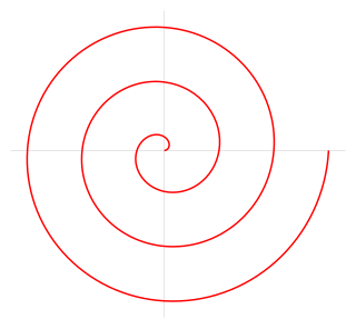
The Archimedean spiral (also known as the arithmetic spiral) is a spiral named after the 3rd-century BC Greek mathematician Archimedes. It is the locus corresponding to the locations over time of a point moving away from a fixed point with a constant speed along a line that rotates with constant angular velocity. Equivalently, in polar coordinates (r, θ) it can be described by the equation
In physics, equations of motion are equations that describe the behavior of a physical system in terms of its motion as a function of time. More specifically, the equations of motion describe the behavior of a physical system as a set of mathematical functions in terms of dynamic variables. These variables are usually spatial coordinates and time, but may include momentum components. The most general choice are generalized coordinates which can be any convenient variables characteristic of the physical system. The functions are defined in a Euclidean space in classical mechanics, but are replaced by curved spaces in relativity. If the dynamics of a system is known, the equations are the solutions for the differential equations describing the motion of the dynamics.
Kinematics is a subfield of physics and mathematics, developed in classical mechanics, that describes the motion of points, bodies (objects), and systems of bodies without considering the forces that cause them to move. Kinematics, as a field of study, is often referred to as the "geometry of motion" and is occasionally seen as a branch of both applied and pure mathematics since it can be studied without considering the mass of a body or the forces acting upon it. A kinematics problem begins by describing the geometry of the system and declaring the initial conditions of any known values of position, velocity and/or acceleration of points within the system. Then, using arguments from geometry, the position, velocity and acceleration of any unknown parts of the system can be determined. The study of how forces act on bodies falls within kinetics, not kinematics. For further details, see analytical dynamics.
In calculus, and more generally in mathematical analysis, integration by parts or partial integration is a process that finds the integral of a product of functions in terms of the integral of the product of their derivative and antiderivative. It is frequently used to transform the antiderivative of a product of functions into an antiderivative for which a solution can be more easily found. The rule can be thought of as an integral version of the product rule of differentiation; it is indeed derived using the product rule.
Chebyshev filters are analog or digital filters that have a steeper roll-off than Butterworth filters, and have either passband ripple or stopband ripple. Chebyshev filters have the property that they minimize the error between the idealized and the actual filter characteristic over the operating frequency range of the filter, but they achieve this with ripples in the passband. This type of filter is named after Pafnuty Chebyshev because its mathematical characteristics are derived from Chebyshev polynomials. Type I Chebyshev filters are usually referred to as "Chebyshev filters", while type II filters are usually called "inverse Chebyshev filters". Because of the passband ripple inherent in Chebyshev filters, filters with a smoother response in the passband but a more irregular response in the stopband are preferred for certain applications.
In physics, circular motion is a movement of an object along the circumference of a circle or rotation along a circular arc. It can be uniform, with a constant rate of rotation and constant tangential speed, or non-uniform with a changing rate of rotation. The rotation around a fixed axis of a three-dimensional body involves the circular motion of its parts. The equations of motion describe the movement of the center of mass of a body, which remains at a constant distance from the axis of rotation. In circular motion, the distance between the body and a fixed point on its surface remains the same, i.e., the body is assumed rigid.
In physics, the Rabi cycle is the cyclic behaviour of a two-level quantum system in the presence of an oscillatory driving field. A great variety of physical processes belonging to the areas of quantum computing, condensed matter, atomic and molecular physics, and nuclear and particle physics can be conveniently studied in terms of two-level quantum mechanical systems, and exhibit Rabi flopping when coupled to an optical driving field. The effect is important in quantum optics, magnetic resonance and quantum computing, and is named after Isidor Isaac Rabi.
In physics, a wave vector is a vector used in describing a wave, with a typical unit being cycle per metre. It has a magnitude and direction. Its magnitude is the wavenumber of the wave, and its direction is perpendicular to the wavefront. In isotropic media, this is also the direction of wave propagation.
A fictitious force is a force that appears to act on a mass whose motion is described using a non-inertial frame of reference, such as a linearly accelerating or rotating reference frame. Fictitious forces are invoked to maintain the validity and thus use of Newton's second law of motion, in frames of reference which are not inertial.
A rotating frame of reference is a special case of a non-inertial reference frame that is rotating relative to an inertial reference frame. An everyday example of a rotating reference frame is the surface of the Earth.
In rotordynamics, the rigid rotor is a mechanical model of rotating systems. An arbitrary rigid rotor is a 3-dimensional rigid object, such as a top. To orient such an object in space requires three angles, known as Euler angles. A special rigid rotor is the linear rotor requiring only two angles to describe, for example of a diatomic molecule. More general molecules are 3-dimensional, such as water, ammonia, or methane.
In calculus, the Leibniz integral rule for differentiation under the integral sign states that for an integral of the form
The reciprocating motion of a non-offset piston connected to a rotating crank through a connecting rod can be expressed by equations of motion. This article shows how these equations of motion can be derived using calculus as functions of angle (angle domain) and of time (time domain).
A pendulum is a body suspended from a fixed support so that it swings freely back and forth under the influence of gravity. When a pendulum is displaced sideways from its resting, equilibrium position, it is subject to a restoring force due to gravity that will accelerate it back towards the equilibrium position. When released, the restoring force acting on the pendulum's mass causes it to oscillate about the equilibrium position, swinging it back and forth. The mathematics of pendulums are in general quite complicated. Simplifying assumptions can be made, which in the case of a simple pendulum allow the equations of motion to be solved analytically for small-angle oscillations.
In geometry, various formalisms exist to express a rotation in three dimensions as a mathematical transformation. In physics, this concept is applied to classical mechanics where rotational kinematics is the science of quantitative description of a purely rotational motion. The orientation of an object at a given instant is described with the same tools, as it is defined as an imaginary rotation from a reference placement in space, rather than an actually observed rotation from a previous placement in space.
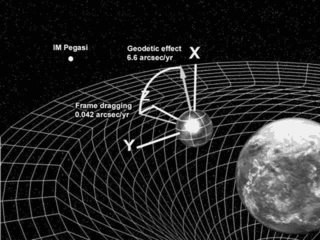
The geodetic effect represents the effect of the curvature of spacetime, predicted by general relativity, on a vector carried along with an orbiting body. For example, the vector could be the angular momentum of a gyroscope orbiting the Earth, as carried out by the Gravity Probe B experiment. The geodetic effect was first predicted by Willem de Sitter in 1916, who provided relativistic corrections to the Earth–Moon system's motion. De Sitter's work was extended in 1918 by Jan Schouten and in 1920 by Adriaan Fokker. It can also be applied to a particular secular precession of astronomical orbits, equivalent to the rotation of the Laplace–Runge–Lenz vector.
In mathematics, the axis–angle representation parameterizes a rotation in a three-dimensional Euclidean space by two quantities: a unit vector e indicating the direction (geometry) of an axis of rotation, and an angle of rotation θ describing the magnitude and sense of the rotation about the axis. Only two numbers, not three, are needed to define the direction of a unit vector e rooted at the origin because the magnitude of e is constrained. For example, the elevation and azimuth angles of e suffice to locate it in any particular Cartesian coordinate frame.
↑ Gaia Collaboration; Drimmel, R.; Romero-Gomez, M.; Chemin, L.; Ramos, P.; Poggio, E.; Ripepi, V.; Andrae, R.; Blomme, R.; Cantat-Gaudin, T.; Castro-Ginard, A. (2022-06-14). "Gaia Data Release 3: Mapping the asymmetric disc of the Milky Way". arXiv:2206.06207 [astro-ph.GA].
↑ pp. 312-321, §4.4, Galactic dynamics (2nd edition), James Binney, Scott Tremaine, Princeton University Press, 2008, ISBN978-0-691-13027-9.
1 2 J. H. Oort (1927-04-14). "Observational evidence confirming Lindblad's hypothesis of a rotation of the galactic system". Bulletin of the Astronomical Institutes of the Netherlands. 3 (120): 275–282. Bibcode:1927BAN.....3..275O.
This page is based on this Wikipedia article Text is available under the CC BY-SA 4.0 license; additional terms may apply. Images, videos and audio are available under their respective licenses.