Vorticity

Last updated

In continuum mechanics, vorticity is a pseudovector field that describes the local spinning motion of a continuum near some point (the tendency of something to rotate [1] ), as would be seen by an observer located at that point and traveling along with the flow. It is an important quantity in the dynamical theory of fluids and provides a convenient framework for understanding a variety of complex flow phenomena, such as the formation and motion of vortex rings. [2] [3]

Contents

Mathematically, the vorticity is the curl of the flow velocity : [4] [3]

where is the nabla operator. Conceptually, could be determined by marking parts of a continuum in a small neighborhood of the point in question, and watching their relative displacements as they move along the flow. The vorticity would be twice the mean angular velocity vector of those particles relative to their center of mass, oriented according to the right-hand rule.

In a two-dimensional flow, is always perpendicular to the plane of the flow, and can therefore be considered a scalar field.

Examples

In a mass of continuum that is rotating like a rigid body, the vorticity is twice the angular velocity vector of that rotation. This is the case, for example, in the central core of a Rankine vortex. [5]

The vorticity may be nonzero even when all particles are flowing along straight and parallel pathlines, if there is shear (that is, if the flow speed varies across streamlines). For example, in the laminar flow within a pipe with constant cross section, all particles travel parallel to the axis of the pipe; but faster near that axis, and practically stationary next to the walls. The vorticity will be zero on the axis, and maximum near the walls, where the shear is largest.

Conversely, a flow may have zero vorticity even though its particles travel along curved trajectories. An example is the ideal irrotational vortex, where most particles rotate about some straight axis, with speed inversely proportional to their distances to that axis. A small parcel of continuum that does not straddle the axis will be rotated in one sense but sheared in the opposite sense, in such a way that their mean angular velocity about their center of mass is zero.

Example flows:
Vorticity Figure 01 a-m.gif Vorticity Figure 03 a-m.gif Vorticity Figure 02 a-m.gif
Rigid-body-like vortex
vr
Parallel flow with shearIrrotational vortex
v1/r
where v is the velocity of the flow, r is the distance to the center of the vortex and ∝ indicates proportionality.
Absolute velocities around the highlighted point:
Vorticity Figure 01 b.png Vorticity Figure 03 b.png Vorticity Figure 02 b.png
Relative velocities (magnified) around the highlighted point
Vorticity Figure 01 c.png Vorticity Figure 03 c.png Vorticity Figure 02 c.png
Vorticity ≠ 0Vorticity ≠ 0Vorticity = 0

Another way to visualize vorticity is to imagine that, instantaneously, a tiny part of the continuum becomes solid and the rest of the flow disappears. If that tiny new solid particle is rotating, rather than just moving with the flow, then there is vorticity in the flow. In the figure below, the left subfigure demonstrates no vorticity, and the right subfigure demonstrates existence of vorticity.

Illustration of vorticity.svg

Mathematical definition

Mathematically, the vorticity of a three-dimensional flow is a pseudovector field, usually denoted by , defined as the curl of the velocity field describing the continuum motion. In Cartesian coordinates:

In words, the vorticity tells how the velocity vector changes when one moves by an infinitesimal distance in a direction perpendicular to it.

In a two-dimensional flow where the velocity is independent of the -coordinate and has no -component, the vorticity vector is always parallel to the -axis, and therefore can be expressed as a scalar field multiplied by a constant unit vector :

The vorticity is also related to the flow's circulation (line integral of the velocity) along a closed path by the (classical) Stokes' theorem. Namely, for any infinitesimal surface element C with normal direction and area , the circulation along the perimeter of is the dot product where is the vorticity at the center of . [6]

Evolution

The evolution of the vorticity field in time is described by the vorticity equation, which can be derived from the Navier–Stokes equations. [7]

In many real flows where the viscosity can be neglected (more precisely, in flows with high Reynolds number), the vorticity field can be modeled by a collection of discrete vortices, the vorticity being negligible everywhere except in small regions of space surrounding the axes of the vortices. This is true in the case of two-dimensional potential flow (i.e. two-dimensional zero viscosity flow), in which case the flowfield can be modeled as a complex-valued field on the complex plane.

Vorticity is useful for understanding how ideal potential flow solutions can be perturbed to model real flows. In general, the presence of viscosity causes a diffusion of vorticity away from the vortex cores into the general flow field; this flow is accounted for by a diffusion term in the vorticity transport equation. [8]

Vortex lines and vortex tubes

A vortex line or vorticity line is a line which is everywhere tangent to the local vorticity vector. Vortex lines are defined by the relation [9]

where is the vorticity vector in Cartesian coordinates.

A vortex tube is the surface in the continuum formed by all vortex lines passing through a given (reducible) closed curve in the continuum. The 'strength' of a vortex tube (also called vortex flux) [10] is the integral of the vorticity across a cross-section of the tube, and is the same everywhere along the tube (because vorticity has zero divergence). It is a consequence of Helmholtz's theorems (or equivalently, of Kelvin's circulation theorem) that in an inviscid fluid the 'strength' of the vortex tube is also constant with time. Viscous effects introduce frictional losses and time dependence. [11]

In a three-dimensional flow, vorticity (as measured by the volume integral of the square of its magnitude) can be intensified when a vortex line is extended — a phenomenon known as vortex stretching. [12] This phenomenon occurs in the formation of a bathtub vortex in outflowing water, and the build-up of a tornado by rising air currents.

Vorticity meters

Rotating-vane vorticity meter

A rotating-vane vorticity meter was invented by Russian hydraulic engineer A. Ya. Milovich (1874–1958). In 1913 he proposed a cork with four blades attached as a device qualitatively showing the magnitude of the vertical projection of the vorticity and demonstrated a motion-picture photography of the float's motion on the water surface in a model of a river bend. [13]

Rotating-vane vorticity meters are commonly shown in educational films on continuum mechanics (famous examples include the NCFMF's "Vorticity" [14] and "Fundamental Principles of Flow" by Iowa Institute of Hydraulic Research [15] ).

Specific sciences

Aeronautics

In aerodynamics, the lift distribution over a finite wing may be approximated by assuming that each spanwise segment of the wing has a semi-infinite trailing vortex behind it. It is then possible to solve for the strength of the vortices using the criterion that there be no flow induced through the surface of the wing. This procedure is called the vortex panel method of computational fluid dynamics. The strengths of the vortices are then summed to find the total approximate circulation about the wing. According to the Kutta–Joukowski theorem, lift per unit of span is the product of circulation, airspeed, and air density.

Atmospheric sciences

The relative vorticity is the vorticity relative to the Earth induced by the air velocity field. This air velocity field is often modeled as a two-dimensional flow parallel to the ground, so that the relative vorticity vector is generally scalar rotation quantity perpendicular to the ground. Vorticity is positive when – looking down onto the Earth's surface – the wind turns counterclockwise. In the northern hemisphere, positive vorticity is called cyclonic rotation, and negative vorticity is anticyclonic rotation; the nomenclature is reversed in the Southern Hemisphere.

The absolute vorticity is computed from the air velocity relative to an inertial frame, and therefore includes a term due to the Earth's rotation, the Coriolis parameter.

The potential vorticity is absolute vorticity divided by the vertical spacing between levels of constant (potential) temperature (or entropy). The absolute vorticity of an air mass will change if the air mass is stretched (or compressed) in the vertical direction, but the potential vorticity is conserved in an adiabatic flow. As adiabatic flow predominates in the atmosphere, the potential vorticity is useful as an approximate tracer of air masses in the atmosphere over the timescale of a few days, particularly when viewed on levels of constant entropy.

The barotropic vorticity equation is the simplest way for forecasting the movement of Rossby waves (that is, the troughs and ridges of 500  hPa geopotential height) over a limited amount of time (a few days). In the 1950s, the first successful programs for numerical weather forecasting utilized that equation.

In modern numerical weather forecasting models and general circulation models (GCMs), vorticity may be one of the predicted variables, in which case the corresponding time-dependent equation is a prognostic equation.

Related to the concept of vorticity is the helicity , defined as

where the integral is over a given volume . In atmospheric science, helicity of the air motion is important in forecasting supercells and the potential for tornadic activity. [16]

See also

Fluid dynamics

Atmospheric sciences

Related Research Articles

<span class="mw-page-title-main">Navier–Stokes equations</span> Equations describing the motion of viscous fluid substances

The Navier–Stokes equations are partial differential equations which describe the motion of viscous fluid substances. They were named after French engineer and physicist Claude-Louis Navier and the Irish physicist and mathematician George Gabriel Stokes. They were developed over several decades of progressively building the theories, from 1822 (Navier) to 1842–1850 (Stokes).

<span class="mw-page-title-main">Potential flow</span> Velocity field as the gradient of a scalar function

In fluid dynamics, potential flow is the ideal flow pattern of an inviscid fluid. Potential flows are described and determined by mathematical methods.

<span class="mw-page-title-main">Vortex</span> Fluid flow revolving around an axis of rotation

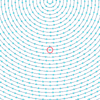
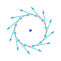
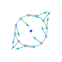
In fluid dynamics, a vortex is a region in a fluid in which the flow revolves around an axis line, which may be straight or curved. Vortices form in stirred fluids, and may be observed in smoke rings, whirlpools in the wake of a boat, and the winds surrounding a tropical cyclone, tornado or dust devil.

The vorticity equation of fluid dynamics describes the evolution of the vorticity ω of a particle of a fluid as it moves with its flow; that is, the local rotation of the fluid. The governing equation is:

<span class="mw-page-title-main">Baroclinity</span> Measure of misalignment between the gradients of pressure and density in a fluid

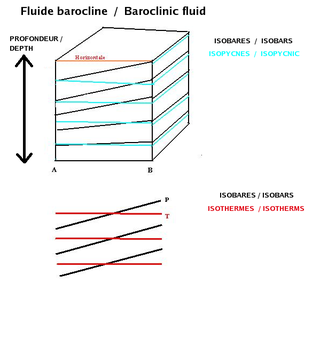
In fluid dynamics, the baroclinity of a stratified fluid is a measure of how misaligned the gradient of pressure is from the gradient of density in a fluid. In meteorology a baroclinic flow is one in which the density depends on both temperature and pressure. A simpler case, barotropic flow, allows for density dependence only on pressure, so that the curl of the pressure-gradient force vanishes.

In fluid dynamics, Stokes' law is an empirical law for the frictional force – also called drag force – exerted on spherical objects with very small Reynolds numbers in a viscous fluid. It was derived by George Gabriel Stokes in 1851 by solving the Stokes flow limit for small Reynolds numbers of the Navier–Stokes equations.

In fluid mechanics, Helmholtz's theorems, named after Hermann von Helmholtz, describe the three-dimensional motion of fluid in the vicinity of vortex lines. These theorems apply to inviscid flows and flows where the influence of viscous forces are small and can be ignored.

In fluid mechanics, the Taylor–Proudman theorem states that when a solid body is moved slowly within a fluid that is steadily rotated with a high angular velocity , the fluid velocity will be uniform along any line parallel to the axis of rotation. must be large compared to the movement of the solid body in order to make the Coriolis force large compared to the acceleration terms.

In fluid dynamics, helicity is, under appropriate conditions, an invariant of the Euler equations of fluid flow, having a topological interpretation as a measure of linkage and/or knottedness of vortex lines in the flow. This was first proved by Jean-Jacques Moreau in 1961 and Moffatt derived it in 1969 without the knowledge of Moreau's paper. This helicity invariant is an extension of Woltjer's theorem for magnetic helicity.

In fluid mechanics, potential vorticity (PV) is a quantity which is proportional to the dot product of vorticity and stratification. This quantity, following a parcel of air or water, can only be changed by diabatic or frictional processes. It is a useful concept for understanding the generation of vorticity in cyclogenesis, especially along the polar front, and in analyzing flow in the ocean.

<span class="mw-page-title-main">Quantum vortex</span> Quantized flux circulation of some physical quantity

In physics, a quantum vortex represents a quantized flux circulation of some physical quantity. In most cases, quantum vortices are a type of topological defect exhibited in superfluids and superconductors. The existence of quantum vortices was first predicted by Lars Onsager in 1949 in connection with superfluid helium. Onsager reasoned that quantisation of vorticity is a direct consequence of the existence of a superfluid order parameter as a spatially continuous wavefunction. Onsager also pointed out that quantum vortices describe the circulation of superfluid and conjectured that their excitations are responsible for superfluid phase transitions. These ideas of Onsager were further developed by Richard Feynman in 1955 and in 1957 were applied to describe the magnetic phase diagram of type-II superconductors by Alexei Alexeyevich Abrikosov. In 1935 Fritz London published a very closely related work on magnetic flux quantization in superconductors. London's fluxoid can also be viewed as a quantum vortex.

The derivation of the Navier–Stokes equations as well as its application and formulation for different families of fluids, is an important exercise in fluid dynamics with applications in mechanical engineering, physics, chemistry, heat transfer, and electrical engineering. A proof explaining the properties and bounds of the equations, such as Navier–Stokes existence and smoothness, is one of the important unsolved problems in mathematics.

The Cauchy momentum equation is a vector partial differential equation put forth by Cauchy that describes the non-relativistic momentum transport in any continuum.

In fluid dynamics, the Oseen equations describe the flow of a viscous and incompressible fluid at small Reynolds numbers, as formulated by Carl Wilhelm Oseen in 1910. Oseen flow is an improved description of these flows, as compared to Stokes flow, with the (partial) inclusion of convective acceleration.

<span class="mw-page-title-main">Mild-slope equation</span> Physics phenomenon and formula

In fluid dynamics, the mild-slope equation describes the combined effects of diffraction and refraction for water waves propagating over bathymetry and due to lateral boundaries—like breakwaters and coastlines. It is an approximate model, deriving its name from being originally developed for wave propagation over mild slopes of the sea floor. The mild-slope equation is often used in coastal engineering to compute the wave-field changes near harbours and coasts.

<span class="mw-page-title-main">Vortex stretching</span> Lengthening of vortices in 3D fluid flow

In fluid dynamics, vortex stretching is the lengthening of vortices in three-dimensional fluid flow, associated with a corresponding increase of the component of vorticity in the stretching direction—due to the conservation of angular momentum.

The viscous vortex domains (VVD) method is a mesh-free method of computational fluid dynamics for directly numerically solving 2D Navier-Stokes equations in Lagrange coordinates. It doesn't implement any turbulence model and free of arbitrary parameters. The main idea of this method is to present vorticity field with discrete regions (domains), which travel with diffusive velocity relatively to fluid and conserve their circulation. The same approach was used in Diffusion Velocity method of Ogami and Akamatsu, but VVD uses other discrete formulas

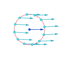
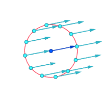
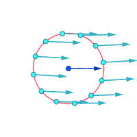
In fluid dynamics, the Burgers vortex or Burgers–Rott vortex is an exact solution to the Navier–Stokes equations governing viscous flow, named after Jan Burgers and Nicholas Rott. The Burgers vortex describes a stationary, self-similar flow. An inward, radial flow, tends to concentrate vorticity in a narrow column around the symmetry axis, while an axial stretching causes the vorticity to increase. At the same time, viscous diffusion tends to spread the vorticity. The stationary Burgers vortex arises when the three effects are in balance.

The Lambda2 method, or Lambda2 vortex criterion, is a vortex core line detection algorithm that can adequately identify vortices from a three-dimensional fluid velocity field. The Lambda2 method is Galilean invariant, which means it produces the same results when a uniform velocity field is added to the existing velocity field or when the field is translated.

In fluid dynamics, Beltrami flows are flows in which the vorticity vector and the velocity vector are parallel to each other. In other words, Beltrami flow is a flow where Lamb vector is zero. It is named after the Italian mathematician Eugenio Beltrami due to his derivation of the Beltrami vector field, while initial developments in fluid dynamics were done by the Russian scientist Ippolit S. Gromeka in 1881.

References

  1. Lecture Notes from University of Washington Archived October 16, 2015, at the Wayback Machine
  2. Moffatt, H.K. (2015), "Fluid Dynamics", in Nicholas J. Higham; et al. (eds.), The Princeton Companion to Applied Mathematics, Princeton University Press, pp. 467–476
  3. 1 2 Guyon, Etienne; Hulin, Jean-Pierre; Petit, Luc; Mitescu, Catalin D. (2001). Physical Hydrodynamics. Oxford University Press. pp. 105, 268–310. ISBN   0-19-851746-7.
  4. Acheson, D.J. (1990). Elementary Fluid Dynamics. Oxford University Press. p. 10. ISBN   0-19-859679-0.
  5. Acheson (1990), p. 15
  6. Clancy, L.J., Aerodynamics, Section 7.11
  7. Guyon, et al (2001), pp. 289–290
  8. Thorne, Kip S.; Blandford, Roger D. (2017). Modern Classical Physics: Optics, Fluids, Plasmas, Elasticity, Relativity, and Statistical Physics. Princeton University Press. p. 741. ISBN   9780691159027.
  9. Kundu P and Cohen I. Fluid Mechanics.
  10. Introduction to Astrophysical Gas Dynamics Archived June 14, 2011, at the Wayback Machine
  11. G.K. Batchelor, An Introduction to Fluid Dynamics (1967), Section 2.6, Cambridge University Press ISBN 0521098173
  12. Batchelor, section 5.2
  13. Joukovsky N.E. (1914). "On the motion of water at a turn of a river". Matematicheskii Sbornik . 28.. Reprinted in: Collected works. Vol. 4. Moscow; Leningrad. 1937. pp. 193–216, 231–233 (abstract in English).{{cite book}}: CS1 maint: location missing publisher (link) "Professor Milovich's float", as Joukovsky refers this vorticity meter to, is schematically shown in figure on page 196 of Collected works.
  14. National Committee for Fluid Mechanics Films Archived October 21, 2016, at the Wayback Machine
  15. Films by Hunter Rouse — IIHR — Hydroscience & Engineering Archived April 21, 2016, at the Wayback Machine
  16. Scheeler, Martin W.; van Rees, Wim M.; Kedia, Hridesh; Kleckner, Dustin; Irvine, William T. M. (2017). "Complete measurement of helicity and its dynamics in vortex tubes". Science. 357 (6350): 487–491. Bibcode:2017Sci...357..487S. doi: 10.1126/science.aam6897 . ISSN   0036-8075. PMID   28774926. S2CID   23287311.

Bibliography

Further reading