This article's lead sectionmay be too short to adequately summarize the key points. Please consider expanding the lead to provide an accessible overview of all important aspects of the article.(July 2015)
The purpose of this page is to provide supplementary materials for the ordinary least squares article, reducing the load of the main article with mathematics and improving its accessibility, while at the same time retaining the completeness of exposition.
Given that S is convex, it is minimized when its gradient vector is zero (This follows by definition: if the gradient vector is not zero, there is a direction in which we can move to minimize it further – see maxima and minima.) The elements of the gradient vector are the partial derivatives of S with respect to the parameters:
The derivatives are
Substitution of the expressions for the residuals and the derivatives into the gradient equations gives
Thus if minimizes S, we have
Upon rearrangement, we obtain the normal equations:
The normal equations are written in matrix notation as
The solution of the normal equations yields the vector of the optimal parameter values.
Derivation directly in terms of matrices
The normal equations can be derived directly from a matrix representation of the problem as follows. The objective is to minimize
Here has the dimension 1x1 (the number of columns of ), so it is a scalar and equal to its own transpose, hence and the quantity to minimize becomes
Differentiating this with respect to and equating to zero to satisfy the first-order conditions gives
which is equivalent to the above-given normal equations. A sufficient condition for satisfaction of the second-order conditions for a minimum is that have full column rank, in which case is positive definite.
Derivation without calculus
When is positive definite, the formula for the minimizing value of can be derived without the use of derivatives. The quantity
can be written as
where depends only on and , and is the inner product defined by
It follows that is equal to
and therefore minimized exactly when
Generalization for complex equations
In general, the coefficients of the matrices and can be complex. By using a Hermitian transpose instead of a simple transpose, it is possible to find a vector which minimizes , just as for the real matrix case. In order to get the normal equations we follow a similar path as in previous derivations:
where stands for Hermitian transpose.
We should now take derivatives of with respect to each of the coefficients , but first we separate real and imaginary parts to deal with the conjugate factors in above expression. For the we have
and the derivatives change into
After rewriting in the summation form and writing explicitly, we can calculate both partial derivatives with result:
which, after adding it together and comparing to zero (minimization condition for ) yields
In matrix form:
Least squares estimator for β
Using matrix notation, the sum of squared residuals is given by
Since this is a quadratic expression, the vector which gives the global minimum may be found via matrix calculus by differentiating with respect to the vector (using denominator layout) and setting equal to zero:
By assumption matrix X has full column rank, and therefore XTX is invertible and the least squares estimator for β is given by
For a simple linear regression model, where ( is the y-intercept and is the slope), one obtains
Expected value and biasedness of
First we will plug in the expression for y into the estimator, and use the fact that X'M=MX=0 (matrix M projects onto the space orthogonal to X):
Now we can recognize ε′Mε as a 1×1 matrix, such matrix is equal to its own trace. This is useful because by properties of trace operator, tr(AB)=tr(BA), and we can use this to separate disturbance ε from matrix M which is a function of regressors X:
Recall that M=I−P where P is the projection onto linear space spanned by columns of matrix X. By properties of a projection matrix, it has p=rank(X) eigenvalues equal to 1, and all other eigenvalues are equal to 0. Trace of a matrix is equal to the sum of its characteristic values, thus tr(P)=p, and tr(M)=n−p. Therefore,
Since the expected value of does not equal the parameter it estimates, , it is a biased estimator of . Note in the later section “Maximum likelihood” we show that under the additional assumption that errors are distributed normally, the estimator is proportional to a chi-squared distribution with n–p degrees of freedom, from which the formula for expected value would immediately follow. However the result we have shown in this section is valid regardless of the distribution of the errors, and thus has importance on its own.
Maximum likelihood estimation is a generic technique for estimating the unknown parameters in a statistical model by constructing a log-likelihood function corresponding to the joint distribution of the data, then maximizing this function over all possible parameter values. In order to apply this method, we have to make an assumption about the distribution of y given X so that the log-likelihood function can be constructed. The connection of maximum likelihood estimation to OLS arises when this distribution is modeled as a multivariate normal.
Specifically, assume that the errors ε have multivariate normal distribution with mean 0 and variance matrix σ2I. Then the distribution of y conditionally on X is
and the log-likelihood function of the data will be
Differentiating this expression with respect to β and σ2 we'll find the ML estimates of these parameters:
We can check that this is indeed a maximum by looking at the Hessian matrix of the log-likelihood function.
Finite-sample distribution
Since we have assumed in this section that the distribution of error terms is known to be normal, it becomes possible to derive the explicit expressions for the distributions of estimators and :
where is the symmetric projection matrix onto subspace orthogonal to X, and thus MX = X′M = 0. We have argued before that this matrix rank n–p, and thus by properties of chi-squared distribution,
Moreover, the estimators and turn out to be independent (conditional on X), a fact which is fundamental for construction of the classical t- and F-tests. The independence can be easily seen from following: the estimator represents coefficients of vector decomposition of by the basis of columns of X, as such is a function of Pε. At the same time, the estimator is a norm of vector Mε divided by n, and thus this estimator is a function of Mε. Now, random variables (Pε, Mε) are jointly normal as a linear transformation of ε, and they are also uncorrelated because PM = 0. By properties of multivariate normal distribution, this means that Pε and Mε are independent, and therefore estimators and will be independent as well.
We look for and that minimize the sum of squared errors (SSE):
To find a minimum take partial derivatives with respect to and
Before taking partial derivative with respect to , substitute the previous result for
Now, take the derivative with respect to :
And finally substitute to determine
Related Research Articles
In probability theory and statistics, the multivariate normal distribution, multivariate Gaussian distribution, or joint normal distribution is a generalization of the one-dimensional (univariate) normal distribution to higher dimensions. One definition is that a random vector is said to be k-variate normally distributed if every linear combination of its k components has a univariate normal distribution. Its importance derives mainly from the multivariate central limit theorem. The multivariate normal distribution is often used to describe, at least approximately, any set of (possibly) correlated real-valued random variables each of which clusters around a mean value.
In statistical mechanics, the Fokker–Planck equation is a partial differential equation that describes the time evolution of the probability density function of the velocity of a particle under the influence of drag forces and random forces, as in Brownian motion. The equation can be generalized to other observables as well.
In statistics, the Gauss–Markov theorem states that the ordinary least squares (OLS) estimator has the lowest sampling variance within the class of linear unbiased estimators, if the errors in the linear regression model are uncorrelated, have equal variances and expectation value of zero. The errors do not need to be normal, nor do they need to be independent and identically distributed. The requirement that the estimator be unbiased cannot be dropped, since biased estimators exist with lower variance. See, for example, the James–Stein estimator, ridge regression, or simply any degenerate estimator.
In continuum mechanics, the infinitesimal strain theory is a mathematical approach to the description of the deformation of a solid body in which the displacements of the material particles are assumed to be much smaller than any relevant dimension of the body; so that its geometry and the constitutive properties of the material at each point of space can be assumed to be unchanged by the deformation.
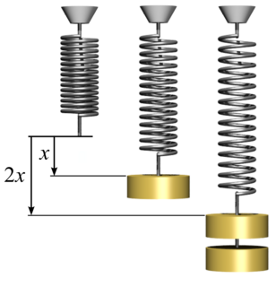
Hooke's law is a law of physics that states that the force needed to extend or compress a spring by some distance scales linearly with respect to that distance—that is, Fs = kx, where k is a constant factor characteristic of the spring, and x is small compared to the total possible deformation of the spring. The law is named after 17th-century British physicist Robert Hooke. He first stated the law in 1676 as a Latin anagram. He published the solution of his anagram in 1678 as: ut tensio, sic vis. Hooke states in the 1678 work that he was aware of the law since 1660.
Linear elasticity is a mathematical model of how solid objects deform and become internally stressed due to prescribed loading conditions. It is a simplification of the more general nonlinear theory of elasticity and a branch of continuum mechanics.
In statistics, a probit model is a type of regression where the dependent variable can take only two values, for example married or not married. The word is a portmanteau, coming from probability + unit. The purpose of the model is to estimate the probability that an observation with particular characteristics will fall into a specific one of the categories; moreover, classifying observations based on their predicted probabilities is a type of binary classification model.
In statistics, ordinary least squares (OLS) is a type of linear least squares method for estimating the unknown parameters in a linear regression model. OLS chooses the parameters of a linear function of a set of explanatory variables by the principle of least squares: minimizing the sum of the squares of the differences between the observed dependent variable in the given dataset and those predicted by the linear function of the independent variable.
Weighted least squares (WLS), also known as weighted linear regression, is a generalization of ordinary least squares and linear regression in which knowledge of the variance of observations is incorporated into the regression. WLS is also a specialization of generalized least squares.
In statistics, simple linear regression is a linear regression model with a single explanatory variable. That is, it concerns two-dimensional sample points with one independent variable and one dependent variable and finds a linear function that, as accurately as possible, predicts the dependent variable values as a function of the independent variable. The adjective simple refers to the fact that the outcome variable is related to a single predictor.
The J-integral represents a way to calculate the strain energy release rate, or work (energy) per unit fracture surface area, in a material. The theoretical concept of J-integral was developed in 1967 by G. P. Cherepanov and independently in 1968 by James R. Rice, who showed that an energetic contour path integral was independent of the path around a crack.
In statistics, Cook's distance or Cook's D is a commonly used estimate of the influence of a data point when performing a least-squares regression analysis. In a practical ordinary least squares analysis, Cook's distance can be used in several ways: to indicate influential data points that are particularly worth checking for validity; or to indicate regions of the design space where it would be good to be able to obtain more data points. It is named after the American statistician R. Dennis Cook, who introduced the concept in 1977.
In statistics, generalized least squares (GLS) is a technique for estimating the unknown parameters in a linear regression model when there is a certain degree of correlation between the residuals in a regression model. In these cases, ordinary least squares and weighted least squares can be statistically inefficient, or even give misleading inferences. GLS was first described by Alexander Aitken in 1936.
In statistics, Bayesian linear regression is an approach to linear regression in which the statistical analysis is undertaken within the context of Bayesian inference. When the regression model has errors that have a normal distribution, and if a particular form of prior distribution is assumed, explicit results are available for the posterior probability distributions of the model's parameters.
In statistics, Bayesian multivariate linear regression is a Bayesian approach to multivariate linear regression, i.e. linear regression where the predicted outcome is a vector of correlated random variables rather than a single scalar random variable. A more general treatment of this approach can be found in the article MMSE estimator.
In linear regression, mean response and predicted response are values of the dependent variable calculated from the regression parameters and a given value of the independent variable. The values of these two responses are the same, but their calculated variances are different.
In statistics, principal component regression (PCR) is a regression analysis technique that is based on principal component analysis (PCA). More specifically, PCR is used for estimating the unknown regression coefficients in a standard linear regression model.
In statistics and in particular in regression analysis, leverage is a measure of how far away the independent variable values of an observation are from those of the other observations. High-leverage points, if any, are outliers with respect to the independent variables. That is, high-leverage points have no neighboring points in space, where is the number of independent variables in a regression model. This makes the fitted model likely to pass close to a high leverage observation. Hence high-leverage points have the potential to cause large changes in the parameter estimates when they are deleted i.e., to be influential points. Although an influential point will typically have high leverage, a high leverage point is not necessarily an influential point. The leverage is typically defined as the diagonal elements of the hat matrix.
The Kirchhoff–Love theory of plates is a two-dimensional mathematical model that is used to determine the stresses and deformations in thin plates subjected to forces and moments. This theory is an extension of Euler-Bernoulli beam theory and was developed in 1888 by Love using assumptions proposed by Kirchhoff. The theory assumes that a mid-surface plane can be used to represent a three-dimensional plate in two-dimensional form.
In statistics, particularly regression analysis, the Working–Hotelling procedure, named after Holbrook Working and Harold Hotelling, is a method of simultaneous estimation in linear regression models. One of the first developments in simultaneous inference, it was devised by Working and Hotelling for the simple linear regression model in 1929. It provides a confidence region for multiple mean responses, that is, it gives the upper and lower bounds of more than one value of a dependent variable at several levels of the independent variables at a certain confidence level. The resulting confidence bands are known as the Working–Hotelling–Scheffé confidence bands.
This page is based on this Wikipedia article Text is available under the CC BY-SA 4.0 license; additional terms may apply. Images, videos and audio are available under their respective licenses.