The quantization of the electromagnetic field means that an electromagnetic field consists of discrete energy parcels called photons. Photons are massless particles of definite energy, definite momentum, and definite spin.
To explain the photoelectric effect, Albert Einstein assumed heuristically in 1905 that an electromagnetic field consists of particles of energy of amount hν, where h is the Planck constant and ν is the wave frequency. In 1927 Paul A. M. Dirac was able to weave the photon concept into the fabric of the new quantum mechanics and to describe the interaction of photons with matter.[1] He applied a technique which is now generally called second quantization,[2] although this term is somewhat of a misnomer for electromagnetic fields, because they are solutions of the classical Maxwell equations. In Dirac's theory the fields are quantized for the first time and it is also the first time that the Planck constant enters the expressions. In his original work, Dirac took the phases of the different electromagnetic modes (Fourier components of the field) and the mode energies as dynamic variables to quantize (i.e., he reinterpreted them as operators and postulated commutation relations between them). At present it is more common to quantize the Fourier components of the vector potential. This is what is done below.
A quantum mechanical photon state belonging to mode is introduced below, and it is shown that it has the following properties:
These equations say respectively: a photon has zero rest mass; the photon energy is hν = hc|k| (k is the wave vector, c is speed of light); its electromagnetic momentum is ħk [ħ = h/(2π)]; the polarization μ = ±1 is the eigenvalue of the z-component of the photon spin.
Second quantization
Second quantization starts with an expansion of a scalar or vector field (or wave functions) in a basis consisting of a complete set of functions. These expansion functions depend on the coordinates of a single particle. The coefficients multiplying the basis functions are interpreted as operators and (anti)commutation relations between these new operators are imposed, commutation relations for bosons and anticommutation relations for fermions (nothing happens to the basis functions themselves). By doing this, the expanded field is converted into a fermion or boson operator field. The expansion coefficients have been promoted from ordinary numbers to operators, creation and annihilation operators. A creation operator creates a particle in the corresponding basis function and an annihilation operator annihilates a particle in this function.
In the case of EM fields the required expansion of the field is the Fourier expansion.
Electromagnetic field and vector potential
As the term suggests, an EM field consists of two vector fields, an electric field and a magnetic field. Both are time-dependent vector fields that in vacuum depend on a third vector field (the vector potential), as well as a scalar field
where denotes the complex conjugate of . The wave vector k gives the propagation direction of the corresponding Fourier component (a polarized monochromatic wave) of A(r,t); the length of the wave vector is
with ν the frequency of the mode. In this summation k runs over all integers, both positive and negative. (The component of Fourier basis is complex conjugate of component of as is real.) The components of the vector k have discrete values (a consequence of the boundary condition that A has the same value on opposite walls of the box):
Two e(μ) ("polarization vectors") are conventional unit vectors for left and right hand circular polarized (LCP and RCP) EM waves (See Jones calculus or Jones vector, Jones calculus) and perpendicular to k. They are related to the orthonormal Cartesian vectors ex and ey through a unitary transformation,
The kth Fourier component of A is a vector perpendicular to k and hence is a linear combination of e(1) and e(−1). The superscript μ indicates a component along e(μ).
Clearly, the (discrete infinite) set of Fourier coefficients and are variables defining the vector potential. In the following they will be promoted to operators.
By using field equations of and in terms of above, electric and magnetic fields are
By using identity ( and are vectors) and as each mode has single frequency dependence.
Quantization of EM field
The best known example of quantization is the replacement of the time-dependent linear momentum of a particle by the rule
Note that the Planck constant is introduced here and that the time-dependence of the classical expression is not taken over in the quantum mechanical operator (this is true in the so-called Schrödinger picture).
For the EM field we do something similar. The quantity is the electric constant, which appears here because of the use of electromagnetic SI units. The quantization rules are:
subject to the boson commutation relations
The square brackets indicate a commutator, defined by for any two quantum mechanical operators A and B. The introduction of the Planck constant is essential in the transition from a classical to a quantum theory. The factor
is introduced to give the Hamiltonian (energy operator) a simple form, see below.
The quantized fields (operator fields) are the following
where ω = c|k| = ck.
Hamiltonian of the field
The classical Hamiltonian has the form
The right-hand-side is easily obtained by first using
(can be derived from Euler equation and trigonometric orthogonality) where k is wavenumber for wave confined within the box of V = L × L × L as described above and second, using ω = kc.
Substitution of the field operators into the classical Hamiltonian gives the Hamilton operator of the EM field,
The second equality follows by use of the third of the boson commutation relations from above with k′ = k and μ′ = μ. Note again that ħω = hν = ħc|k| and remember that ω depends on k, even though it is not explicit in the notation. The notation ω(k) could have been introduced, but is not common as it clutters the equations.
Digression: harmonic oscillator
The second quantized treatment of the one-dimensional quantum harmonic oscillator is a well-known topic in quantum mechanical courses. We digress and say a few words about it. The harmonic oscillator Hamiltonian has the form
where ω≡ 2πν is the fundamental frequency of the oscillator. The ground state of the oscillator is designated by ; and is referred to as the "vacuum state". It can be shown that is an excitation operator, it excites from an n fold excited state to an n + 1 fold excited state:
In particular: and
Since harmonic oscillator energies are equidistant, the n-fold excited state ; can be looked upon as a single state containing n particles (sometimes called vibrons) all of energy hν. These particles are bosons. For obvious reason the excitation operator is called a creation operator.
From the commutation relation follows that the Hermitian adjoint de-excites: in particular so that For obvious reason the de-excitation operator is called an annihilation operator.
By mathematical induction the following "differentiation rule", that will be needed later, is easily proved,
Suppose now we have a number of non-interacting (independent) one-dimensional harmonic oscillators, each with its own fundamental frequency ωi . Because the oscillators are independent, the Hamiltonian is a simple sum:
By substituting for we see that the Hamiltonian of the EM field can be considered a Hamiltonian of independent oscillators of energy ω = |k|c oscillating along direction e(μ) with μ = ±1.
Photon number states (Fock states)
The quantized EM field has a vacuum (no photons) state . The application of it to, say,
gives a quantum state of m photons in mode (k, μ) and n photons in mode (k′, μ′). The proportionality symbol is used because the state on the left-hand is not normalized to unity, whereas the state on the right-hand may be normalized.
The operator
is the number operator. When acting on a quantum mechanical photon number state, it returns the number of photons in mode (k, μ). This also holds when the number of photons in this mode is zero, then the number operator returns zero. To show the action of the number operator on a one-photon ket, we consider
i.e., a number operator of mode (k, μ) returns zero if the mode is unoccupied and returns unity if the mode is singly occupied. To consider the action of the number operator of mode (k, μ) on a n-photon ket of the same mode, we drop the indices k and μ and consider
Use the "differentiation rule" introduced earlier and it follows that
A photon number state (or a Fock state) is an eigenstate of the number operator. This is why the formalism described here is often referred to as the occupation number representation.
Photon energy
Earlier the Hamiltonian,
was introduced. The zero of energy can be shifted, which leads to an expression in terms of the number operator,
The effect of H on a single-photon state is
Apparently, the single-photon state is an eigenstate of H and ħω = hν is the corresponding energy. In the same way
Example photon density
The electromagnetic energy density created by a 100kW radio transmitting station is computed in the article on the electromagnetic wave (where?); the energy density estimate at 5km from the station was 2.1×10⁻¹⁰J/m3. Is quantum mechanics needed to describe the station's broadcast?
The classical approximation to EM radiation is good when the number of photons is much larger than unity in the volume where λ is the length of the radio waves. In that case quantum fluctuations are negligible and cannot be heard.
Suppose the radio station broadcasts at ν = 100MHz, then it is sending out photons with an energy content of νh = 1×108 × 6.6×10−34 = 6.6×10⁻²⁶J, where h is the Planck constant. The wavelength of the station is λ = c/ν = 3m, so that λ/(2π) = 48cm and the volume is 0.109m3. The energy content of this volume element is 2.1×10−10 × 0.109 = 2.3×10⁻¹¹J, which amounts to 3.4×10¹⁴ photons per Obviously, 3.4×10¹⁴ > 1 and hence quantum effects do not play a role; the waves emitted by this station are well-described by the classical limit and quantum mechanics is not needed.
Photon momentum
Introducing the Fourier expansion of the electromagnetic field into the classical form
yields
Quantization gives
The term 1/2 could be dropped, because when one sums over the allowed k, k cancels with −k. The effect of PEM on a single-photon state is
Apparently, the single-photon state is an eigenstate of the momentum operator, and ħk is the eigenvalue (the momentum of a single photon).
Photon mass
The photon having non-zero linear momentum, one could imagine that it has a non-vanishing rest mass m0, which is its mass at zero speed. However, we will now show that this is not the case: m0 = 0.
Since the photon propagates with the speed of light, special relativity is called for. The relativistic expressions for energy and momentum squared are,
From p2/E2,
Use
and it follows that
so that m0 = 0.
Photon spin
The photon can be assigned a triplet spin with spin quantum number S = 1. This is similar to, say, the nuclear spin of the 14N isotope, but with the important difference that the state with MS = 0 is zero, only the states with MS = ±1 are non-zero.
Define spin operators:
The two operators between the two orthogonal unit vectors are dyadic products. The unit vectors are perpendicular to the propagation direction k (the direction of the z axis, which is the spin quantization axis).
The spin operators satisfy the usual angular momentum commutation relations
Indeed, use the dyadic product property
because ez is of unit length. In this manner,
By inspection it follows that
and therefore μ labels the photon spin,
Because the vector potential A is a transverse field, the photon has no forward (μ = 0) spin component.
In quantum mechanics, the Hamiltonian of a system is an operator corresponding to the total energy of that system, including both kinetic energy and potential energy. Its spectrum, the system's energy spectrum or its set of energy eigenvalues, is the set of possible outcomes obtainable from a measurement of the system's total energy. Due to its close relation to the energy spectrum and time-evolution of a system, it is of fundamental importance in most formulations of quantum theory.
In theoretical physics, quantum field theory (QFT) is a theoretical framework that combines classical field theory, special relativity, and quantum mechanics. QFT is used in particle physics to construct physical models of subatomic particles and in condensed matter physics to construct models of quasiparticles.
The quantum harmonic oscillator is the quantum-mechanical analog of the classical harmonic oscillator. Because an arbitrary smooth potential can usually be approximated as a harmonic potential at the vicinity of a stable equilibrium point, it is one of the most important model systems in quantum mechanics. Furthermore, it is one of the few quantum-mechanical systems for which an exact, analytical solution is known.
In physics, specifically in quantum mechanics, a coherent state is the specific quantum state of the quantum harmonic oscillator, often described as a state that has dynamics most closely resembling the oscillatory behavior of a classical harmonic oscillator. It was the first example of quantum dynamics when Erwin Schrödinger derived it in 1926, while searching for solutions of the Schrödinger equation that satisfy the correspondence principle. The quantum harmonic oscillator arise in the quantum theory of a wide range of physical systems. For instance, a coherent state describes the oscillating motion of a particle confined in a quadratic potential well. The coherent state describes a state in a system for which the ground-state wavepacket is displaced from the origin of the system. This state can be related to classical solutions by a particle oscillating with an amplitude equivalent to the displacement.
In mathematics, the Hodge star operator or Hodge star is a linear map defined on the exterior algebra of a finite-dimensional oriented vector space endowed with a nondegenerate symmetric bilinear form. Applying the operator to an element of the algebra produces the Hodge dual of the element. This map was introduced by W. V. D. Hodge.
In differential geometry, the four-gradient is the four-vector analogue of the gradient from vector calculus.
In quantum mechanics, a two-state system is a quantum system that can exist in any quantum superposition of two independent quantum states. The Hilbert space describing such a system is two-dimensional. Therefore, a complete basis spanning the space will consist of two independent states. Any two-state system can also be seen as a qubit.
The Franz–Keldysh effect is a change in optical absorption by a semiconductor when an electric field is applied. The effect is named after the German physicist Walter Franz and Russian physicist Leonid Keldysh.
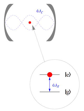
The Jaynes–Cummings model is a theoretical model in quantum optics. It describes the system of a two-level atom interacting with a quantized mode of an optical cavity, with or without the presence of light. It was originally developed to study the interaction of atoms with the quantized electromagnetic field in order to investigate the phenomena of spontaneous emission and absorption of photons in a cavity.
Photon polarization is the quantum mechanical description of the classical polarized sinusoidal plane electromagnetic wave. An individual photon can be described as having right or left circular polarization, or a superposition of the two. Equivalently, a photon can be described as having horizontal or vertical linear polarization, or a superposition of the two.
The theoretical and experimental justification for the Schrödinger equation motivates the discovery of the Schrödinger equation, the equation that describes the dynamics of nonrelativistic particles. The motivation uses photons, which are relativistic particles with dynamics described by Maxwell's equations, as an analogue for all types of particles.
In many-body theory, the term Green's function is sometimes used interchangeably with correlation function, but refers specifically to correlators of field operators or creation and annihilation operators.
In quantum mechanics and quantum field theory, a Schrödinger field, named after Erwin Schrödinger, is a quantum field which obeys the Schrödinger equation. While any situation described by a Schrödinger field can also be described by a many-body Schrödinger equation for identical particles, the field theory is more suitable for situations where the particle number changes.
Surface-extended X-ray absorption fine structure (SEXAFS) is the surface-sensitive equivalent of the EXAFS technique. This technique involves the illumination of the sample by high-intensity X-ray beams from a synchrotron and monitoring their photoabsorption by detecting in the intensity of Auger electrons as a function of the incident photon energy. Surface sensitivity is achieved by the interpretation of data depending on the intensity of the Auger electrons instead of looking at the relative absorption of the X-rays as in the parent method, EXAFS.
In linear algebra, a raising or lowering operator is an operator that increases or decreases the eigenvalue of another operator. In quantum mechanics, the raising operator is sometimes called the creation operator, and the lowering operator the annihilation operator. Well-known applications of ladder operators in quantum mechanics are in the formalisms of the quantum harmonic oscillator and angular momentum.
The neutrino theory of light is the proposal that the photon is a composite particle formed of a neutrino–antineutrino pair. It is based on the idea that emission and absorption of a photon corresponds to the creation and annihilation of a particle–antiparticle pair. The neutrino theory of light is not currently accepted as part of mainstream physics, as according to the Standard Model the photon is an elementary particle, a gauge boson.
Symmetries in quantum mechanics describe features of spacetime and particles which are unchanged under some transformation, in the context of quantum mechanics, relativistic quantum mechanics and quantum field theory, and with applications in the mathematical formulation of the standard model and condensed matter physics. In general, symmetry in physics, invariance, and conservation laws, are fundamentally important constraints for formulating physical theories and models. In practice, they are powerful methods for solving problems and predicting what can happen. While conservation laws do not always give the answer to the problem directly, they form the correct constraints and the first steps to solving a multitude of problems.
In machine learning, the kernel embedding of distributions comprises a class of nonparametric methods in which a probability distribution is represented as an element of a reproducing kernel Hilbert space (RKHS). A generalization of the individual data-point feature mapping done in classical kernel methods, the embedding of distributions into infinite-dimensional feature spaces can preserve all of the statistical features of arbitrary distributions, while allowing one to compare and manipulate distributions using Hilbert space operations such as inner products, distances, projections, linear transformations, and spectral analysis. This learning framework is very general and can be applied to distributions over any space on which a sensible kernel function may be defined. For example, various kernels have been proposed for learning from data which are: vectors in , discrete classes/categories, strings, graphs/networks, images, time series, manifolds, dynamical systems, and other structured objects. The theory behind kernel embeddings of distributions has been primarily developed by Alex Smola, Le Song , Arthur Gretton, and Bernhard Schölkopf. A review of recent works on kernel embedding of distributions can be found in.
In mathematical physics, the Gordon decomposition of the Dirac current is a splitting of the charge or particle-number current into a part that arises from the motion of the center of mass of the particles and a part that arises from gradients of the spin density. It makes explicit use of the Dirac equation and so it applies only to "on-shell" solutions of the Dirac equation.
In quantum computing, Mølmer–Sørensen gate scheme refers to an implementation procedure for various multi-qubit quantum logic gates used mostly in trapped ion quantum computing. This procedure is based on the original proposition by Klaus Mølmer and Anders Sørensen in 1999-2000.
↑ P. A. M. Dirac, The Quantum Theory of the Emission and Absorption of Radiation, Proc. Royal Soc. Lond. A 114, pp. 243–265, (1927) Online (pdf)
↑ The name derives from the second quantization of quantum mechanical wave functions. Such a wave function is a scalar field (the "Schrödinger field") and can be quantized in the very same way as electromagnetic fields. Since a wave function is derived from a "first" quantizedHamiltonian, the quantization of the Schrödinger field is the second time quantization is performed, hence the name.
This page is based on this Wikipedia article Text is available under the CC BY-SA 4.0 license; additional terms may apply. Images, videos and audio are available under their respective licenses.