Ratio of distance on a map to the corresponding distance on the ground
This article is about the general mapping concept. For its graphical representation, see Linear scale. For other uses, see Scale.
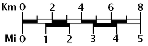
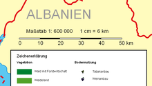
A graphical or bar scale. A map would also usually give its scale numerically ("1:50,000", for instance, means that one cm on the map represents 50,000cm of real space, which is 500 meters)A bar scale with the nominal scale expressed as "1:600 000", meaning 1 cm on the map corresponds to 600,000cm=6km on the ground.
The scale of a map is the ratio of a distance on the map to the corresponding distance on the ground. This simple concept is complicated by the curvature of the Earth's surface, which forces scale to vary across a map. Because of this variation, the concept of scale becomes meaningful in two distinct ways.
The first way is the ratio of the size of the generating globe to the size of the Earth. The generating globe is a conceptual model to which the Earth is shrunk and from which the map is projected. The ratio of the Earth's size to the generating globe's size is called the nominal scale (also called principal scale or representative fraction). Many maps state the nominal scale and may even display a bar scale (sometimes merely called a "scale") to represent it.
The second distinct concept of scale applies to the variation in scale across a map. It is the ratio of the mapped point's scale to the nominal scale. In this case 'scale' means the scale factor (also called point scale or particular scale).
If the region of the map is small enough to ignore Earth's curvature, such as in a town plan, then a single value can be used as the scale without causing measurement errors. In maps covering larger areas, or the whole Earth, the map's scale may be less useful or even useless in measuring distances. The map projection becomes critical in understanding how scale varies throughout the map.[1][2] When scale varies noticeably, it can be accounted for as the scale factor. Tissot's indicatrix is often used to illustrate the variation of point scale across a map.
History
The foundations for quantitative map scaling goes back to ancient China with textual evidence that the idea of map scaling was understood by the second century BC. Ancient Chinese surveyors and cartographers had ample technical resources used to produce maps such as counting rods, carpenter's square's, plumb lines, compasses for drawing circles, and sighting tubes for measuring inclination. Reference frames postulating a nascent coordinate system for identifying locations were hinted by ancient Chinese astronomers that divided the sky into various sectors or lunar lodges.[3]
The Chinese cartographer and geographer Pei Xiu of the Three Kingdoms period created a set of large-area maps that were drawn to scale. He produced a set of principles that stressed the importance of consistent scaling, directional measurements, and adjustments in land measurements in the terrain that was being mapped.[3]
Terminology
Representation of scale
Map scales may be expressed in words (a lexical scale), as a ratio, or as a fraction. Examples are:
'one centimetre to one hundred metres' or 1:10,000 or 1/10,000
'one inch to one mile' or 1:63,360 or 1/63,360
'one centimetre to one thousand kilometres' or 1:100,000,000 or 1/100,000,000. (The ratio would usually be abbreviated to 1:100M)
Bar scale vs. lexical scale
In addition to the above many maps carry one or more (graphical)bar scales. For example, some modern British maps have three bar scales, one each for kilometres, miles and nautical miles.
A lexical scale in a language known to the user may be easier to visualise than a ratio: if the scale is an inch to two miles and the map user can see two villages that are about two inches apart on the map, then it is easy to work out that the villages are about four miles apart on the ground.
A lexical scale may cause problems if it expressed in a language that the user does not understand or in obsolete or ill-defined units. For example, a scale of one inch to a furlong (1:7920) will be understood by many older people in countries where Imperial units used to be taught in schools. But a scale of one pouce to one league may be about 1:144,000, depending on the cartographer's choice of the many possible definitions for a league, and only a minority of modern users will be familiar with the units used.
A small-scale map cover large regions, such as world maps, continents or large nations. In other words, they show large areas of land on a small space. They are called small scale because the representative fraction is relatively small.
Large-scale maps show smaller areas in more detail, such as county maps or town plans might. Such maps are called large scale because the representative fraction is relatively large. For instance a town plan, which is a large-scale map, might be on a scale of 1:10,000, whereas the world map, which is a small scale map, might be on a scale of 1:100,000,000.
The following table describes typical ranges for these scales but should not be considered authoritative because there is no standard:
Classification
Range
Examples
large scale
1:0 – 1:600,000
1:0.00001 for map of virus; 1:5,000 for walking map of town
medium scale
1:600,000 – 1:2,000,000
Map of a country
small scale
1:2,000,000 – 1:∞
1:50,000,000 for world map; 1:1021 for map of galaxy
The terms are sometimes used in the absolute sense of the table, but other times in a relative sense. For example, a map reader whose work refers solely to large-scale maps (as tabulated above) might refer to a map at 1:500,000 as small-scale.
In the English language, the word large-scale is often used to mean "extensive". However, as explained above, cartographers use the term "large scale" to refer to less extensive maps – those that show a smaller area. Maps that show an extensive area are "small scale" maps. This can be a cause of confusion.
Scale variation
Mapping large areas causes noticeable distortions because it significantly flattens the curved surface of the earth. How distortion gets distributed depends on the map projection. Scale varies across the map, and the stated map scale is only an approximation. This is discussed in detail below.
Large-scale maps with curvature neglected
The region over which the earth can be regarded as flat depends on the accuracy of the survey measurements. If measured only to the nearest metre, then curvature of the earth is undetectable over a meridian distance of about 100 kilometres (62mi) and over an east-west line of about 80km (at a latitude of 45 degrees). If surveyed to the nearest 1 millimetre (0.039in), then curvature is undetectable over a meridian distance of about 10km and over an east-west line of about 8km.[4] Thus a plan of New York City accurate to one metre or a building site plan accurate to one millimetre would both satisfy the above conditions for the neglect of curvature. They can be treated by plane surveying and mapped by scale drawings in which any two points at the same distance on the drawing are at the same distance on the ground. True ground distances are calculated by measuring the distance on the map and then multiplying by the inverse of the scale fraction or, equivalently, simply using dividers to transfer the separation between the points on the map to a bar scale on the map.
As proved by Gauss’s Theorema Egregium, a sphere (or ellipsoid) cannot be projected onto a plane without distortion. This is commonly illustrated by the impossibility of smoothing an orange peel onto a flat surface without tearing and deforming it. The only true representation of a sphere at constant scale is another sphere such as a globe.
Given the limited practical size of globes, we must use maps for detailed mapping. Maps require projections. A projection implies distortion: A constant separation on the map does not correspond to a constant separation on the ground. While a map may display a graphical bar scale, the scale must be used with the understanding that it will be accurate on only some lines of the map. (This is discussed further in the examples in the following sections.)
Let P be a point at latitude and longitude on the sphere (or ellipsoid). Let Q be a neighbouring point and let be the angle between the element PQ and the meridian at P: this angle is the azimuth angle of the element PQ. Let P' and Q' be corresponding points on the projection. The angle between the direction P'Q' and the projection of the meridian is the bearing. In general . Comment: this precise distinction between azimuth (on the Earth's surface) and bearing (on the map) is not universally observed, many writers using the terms almost interchangeably.
Definition: the point scale at P is the ratio of the two distances P'Q' and PQ in the limit that Q approaches P. We write this as
where the notation indicates that the point scale is a function of the position of P and also the direction of the element PQ.
Definition: if P and Q lie on the same meridian , the meridian scale is denoted by .
Definition: if P and Q lie on the same parallel , the parallel scale is denoted by .
Definition: if the point scale depends only on position, not on direction, we say that it is isotropic and conventionally denote its value in any direction by the parallel scale factor .
Definition: A map projection is said to be conformal if the angle between a pair of lines intersecting at a point P is the same as the angle between the projected lines at the projected point P', for all pairs of lines intersecting at point P. A conformal map has an isotropic scale factor. Conversely isotropic scale factors across the map imply a conformal projection.
Isotropy of scale implies that small elements are stretched equally in all directions, that is the shape of a small element is preserved. This is the property of orthomorphism (from Greek 'right shape'). The qualification 'small' means that at some given accuracy of measurement no change can be detected in the scale factor over the element. Since conformal projections have an isotropic scale factor they have also been called orthomorphic projections. For example, the Mercator projection is conformal since it is constructed to preserve angles and its scale factor is isotropic, a function of latitude only: Mercator does preserve shape in small regions.
Definition: on a conformal projection with an isotropic scale, points which have the same scale value may be joined to form the isoscale lines. These are not plotted on maps for end users but they feature in many of the standard texts. (See Snyder[1] pages 203—206.)
The representative fraction (RF) or principal scale
There are two conventions used in setting down the equations of any given projection. For example, the equirectangular cylindrical projection may be written as
cartographers:
mathematicians:
Here we shall adopt the first of these conventions (following the usage in the surveys by Snyder). Clearly the above projection equations define positions on a huge cylinder wrapped around the Earth and then unrolled. We say that these coordinates define the projection map which must be distinguished logically from the actual printed (or viewed) maps. If the definition of point scale in the previous section is in terms of the projection map then we can expect the scale factors to be close to unity. For normal tangent cylindrical projections the scale along the equator is k=1 and in general the scale changes as we move off the equator. Analysis of scale on the projection map is an investigation of the change of k away from its true value of unity.
Actual printed maps are produced from the projection map by a constant scaling denoted by a ratio such as 1:100M (for whole world maps) or 1:10000 (for such as town plans). To avoid confusion in the use of the word 'scale' this constant scale fraction is called the representative fraction (RF) of the printed map and it is to be identified with the ratio printed on the map. The actual printed map coordinates for the equirectangular cylindrical projection are
printed map:
This convention allows a clear distinction of the intrinsic projection scaling and the reduction scaling.
From this point we ignore the RF and work with the projection map.
Visualisation of point scale: the Tissot indicatrix
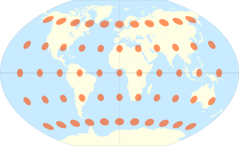
Consider a small circle on the surface of the Earth centred at a point P at latitude and longitude . Since the point scale varies with position and direction the projection of the circle on the projection will be distorted. Tissot proved that, as long as the distortion is not too great, the circle will become an ellipse on the projection. In general the dimension, shape and orientation of the ellipse will change over the projection. Superimposing these distortion ellipses on the map projection conveys the way in which the point scale is changing over the map. The distortion ellipse is known as Tissot's indicatrix. The example shown here is the Winkel tripel projection, the standard projection for world maps made by the National Geographic Society. The minimum distortion is on the central meridian at latitudes of 30 degrees (North and South). (Other examples[5][6]).
Point scale for normal cylindrical projections of the sphere
The key to a quantitative understanding of scale is to consider an infinitesimal element on the sphere. The figure shows a point P at latitude and longitude on the sphere. The point Q is at latitude and longitude . The lines PK and MQ are arcs of meridians of length where is the radius of the sphere and is in radian measure. The lines PM and KQ are arcs of parallel circles of length with in radian measure. In deriving a point property of the projection at P it suffices to take an infinitesimal element PMQK of the surface: in the limit of Q approaching P such an element tends to an infinitesimally small planar rectangle.
Infinitesimal elements on the sphere and a normal cylindrical projection
Normal cylindrical projections of the sphere have and equal to a function of latitude only. Therefore, the infinitesimal element PMQK on the sphere projects to an infinitesimal element P'M'Q'K' which is an exact rectangle with a base and height. By comparing the elements on sphere and projection we can immediately deduce expressions for the scale factors on parallels and meridians. (The treatment of scale in a general direction may be found below.)
parallel scale factor
meridian scale factor
Note that the parallel scale factor is independent of the definition of so it is the same for all normal cylindrical projections. It is useful to note that
at latitude 30 degrees the parallel scale is
at latitude 45 degrees the parallel scale is
at latitude 60 degrees the parallel scale is
at latitude 80 degrees the parallel scale is
at latitude 85 degrees the parallel scale is
The following examples illustrate three normal cylindrical projections and in each case the variation of scale with position and direction is illustrated by the use of Tissot's indicatrix.
The equirectangular projection,[1][2][4] also known as the Plate Carrée (French for "flat square") or (somewhat misleadingly) the equidistant projection, is defined by
where is the radius of the sphere, is the longitude from the central meridian of the projection (here taken as the Greenwich meridian at ) and is the latitude. Note that and are in radians (obtained by multiplying the degree measure by a factor of /180). The longitude is in the range and the latitude is in the range .
Since the previous section gives
parallel scale,
meridian scale
For the calculation of the point scale in an arbitrary direction see addendum.
The figure illustrates the Tissot indicatrix for this projection. On the equator h=k=1 and the circular elements are undistorted on projection. At higher latitudes the circles are distorted into an ellipse given by stretching in the parallel direction only: there is no distortion in the meridian direction. The ratio of the major axis to the minor axis is . Clearly the area of the ellipse increases by the same factor.
It is instructive to consider the use of bar scales that might appear on a printed version of this projection. The scale is true (k=1) on the equator so that multiplying its length on a printed map by the inverse of the RF (or principal scale) gives the actual circumference of the Earth. The bar scale on the map is also drawn at the true scale so that transferring a separation between two points on the equator to the bar scale will give the correct distance between those points. The same is true on the meridians. On a parallel other than the equator the scale is so when we transfer a separation from a parallel to the bar scale we must divide the bar scale distance by this factor to obtain the distance between the points when measured along the parallel (which is not the true distance along a great circle). On a line at a bearing of say 45 degrees () the scale is continuously varying with latitude and transferring a separation along the line to the bar scale does not give a distance related to the true distance in any simple way. (But see addendum). Even if a distance along this line of constant planar angle could be worked out, its relevance is questionable since such a line on the projection corresponds to a complicated curve on the sphere. For these reasons bar scales on small-scale maps must be used with extreme caution.
Mercator projection
The Mercator projection with Tissot's indicatrix of deformation. (The distortion increases without limit at higher latitudes)
The Mercator projection maps the sphere to a rectangle (of infinite extent in the -direction) by the equations[1][2][4]
where a, and are as in the previous example. Since the scale factors are:
parallel scale
meridian scale
In the mathematical addendum it is shown that the point scale in an arbitrary direction is also equal to so the scale is isotropic (same in all directions), its magnitude increasing with latitude as . In the Tissot diagram each infinitesimal circular element preserves its shape but is enlarged more and more as the latitude increases.
Lambert's equal area projection
Lambert's normal cylindrical equal-area projection with Tissot's indicatrix of deformation
where a, and are as in the previous example. Since the scale factors are
parallel scale
meridian scale
The calculation of the point scale in an arbitrary direction is given below.
The vertical and horizontal scales now compensate each other (hk=1) and in the Tissot diagram each infinitesimal circular element is distorted into an ellipse of the same area as the undistorted circles on the equator.
Graphs of scale factors
The graph shows the variation of the scale factors for the above three examples. The top plot shows the isotropic Mercator scale function: the scale on the parallel is the same as the scale on the meridian. The other plots show the meridian scale factor for the Equirectangular projection (h=1) and for the Lambert equal area projection. These last two projections have a parallel scale identical to that of the Mercator plot. For the Lambert note that the parallel scale (as Mercator A) increases with latitude and the meridian scale (C) decreases with latitude in such a way that hk=1, guaranteeing area conservation.
Scale variation on the Mercator projection
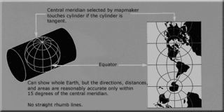
The Mercator point scale is unity on the equator because it is such that the auxiliary cylinder used in its construction is tangential to the Earth at the equator. For this reason the usual projection should be called a tangent projection. The scale varies with latitude as . Since tends to infinity as we approach the poles the Mercator map is grossly distorted at high latitudes and for this reason the projection is totally inappropriate for world maps (unless we are discussing navigation and rhumb lines). However, at a latitude of about 25 degrees the value of is about 1.1 so Mercator is accurate to within 10% in a strip of width 50 degrees centred on the equator. Narrower strips are better: a strip of width 16 degrees (centred on the equator) is accurate to within 1% or 1 part in 100.
A standard criterion for good large-scale maps is that the accuracy should be within 4 parts in 10,000, or 0.04%, corresponding to . Since attains this value at degrees (see figure below, red line). Therefore, the tangent Mercator projection is highly accurate within a strip of width 3.24 degrees centred on the equator. This corresponds to north-south distance of about 360km (220mi). Within this strip Mercator is very good, highly accurate and shape preserving because it is conformal (angle preserving). These observations prompted the development of the transverse Mercator projections in which a meridian is treated 'like an equator' of the projection so that we obtain an accurate map within a narrow distance of that meridian. Such maps are good for countries aligned nearly north-south (like Great Britain) and a set of 60 such maps is used for the Universal Transverse Mercator (UTM). Note that in both these projections (which are based on various ellipsoids) the transformation equations for x and y and the expression for the scale factor are complicated functions of both latitude and longitude.
Scale variation near the equator for the tangent (red) and secant (green) Mercator projections.
Secant, or modified, projections
Comparison of tangent and secant cylindrical, conic and azimuthal map projections with standard parallels shown in red
The basic idea of a secant projection is that the sphere is projected to a cylinder which intersects the sphere at two parallels, say north and south. Clearly the scale is now true at these latitudes whereas parallels beneath these latitudes are contracted by the projection and their (parallel) scale factor must be less than one. The result is that deviation of the scale from unity is reduced over a wider range of latitudes.
As an example, one possible secant Mercator projection is defined by
The numeric multipliers do not alter the shape of the projection but it does mean that the scale factors are modified:
secant Mercator scale,
Thus
the scale on the equator is 0.9996,
the scale is k=1 at a latitude given by where so that degrees,
k=1.0004 at a latitude given by for which degrees. Therefore, the projection has , that is an accuracy of 0.04%, over a wider strip of 4.58 degrees (compared with 3.24 degrees for the tangent form).
This is illustrated by the lower (green) curve in the figure of the previous section.
Such narrow zones of high accuracy are used in the UTM and the British OSGB projection, both of which are secant, transverse Mercator on the ellipsoid with the scale on the central meridian constant at . The isoscale lines with are slightly curved lines approximately 180km east and west of the central meridian. The maximum value of the scale factor is 1.001 for UTM and 1.0007 for OSGB.
The lines of unit scale at latitude (north and south), where the cylindrical projection surface intersects the sphere, are the standard parallels of the secant projection.
Whilst a narrow band with is important for high accuracy mapping at a large scale, for world maps much wider spaced standard parallels are used to control the scale variation. Examples are
Behrmann with standard parallels at 30N, 30S.
Gall equal area with standard parallels at 45N, 45S.
Scale variation for the Lambert (green) and Gall (red) equal area projections.
The scale plots for the latter are shown below compared with the Lambert equal area scale factors. In the latter the equator is a single standard parallel and the parallel scale increases from k=1 to compensate the decrease in the meridian scale. For the Gall the parallel scale is reduced at the equator (to k=0.707) whilst the meridian scale is increased (to k=1.414). This gives rise to the gross distortion of shape in the Gall-Peters projection. (On the globe Africa is about as long as it is broad). Note that the meridian and parallel scales are both unity on the standard parallels.
Mathematical addendum
Infinitesimal elements on the sphere and a normal cylindrical projection
For normal cylindrical projections the geometry of the infinitesimal elements gives
The relationship between the angles and is
For the Mercator projection giving : angles are preserved. (Hardly surprising since this is the relation used to derive Mercator). For the equidistant and Lambert projections we have and respectively so the relationship between and depends upon the latitude. Denote the point scale at P when the infinitesimal element PQ makes an angle with the meridian by It is given by the ratio of distances:
Setting and substituting and from equations (a) and (b) respectively gives
For the projections other than Mercator we must first calculate from and using equation (c), before we can find . For example, the equirectangular projection has so that
If we consider a line of constant slope on the projection both the corresponding value of and the scale factor along the line are complicated functions of . There is no simple way of transferring a general finite separation to a bar scale and obtaining meaningful results.
Ratio symbol
While the colon is often used to express ratios, Unicode can express a symbol specific to ratios, being slightly raised: U+2236∶RATIO (∶).
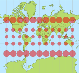
The Mercator projection is a conformal cylindrical map projection presented by Flemish geographer and cartographer Gerardus Mercator in 1569. It became the standard map projection for navigation due to its ability to represent north as 'up' and south as 'down' everywhere while preserving local directions and shapes. However, as a result, the Mercator projection inflates the size of objects the further they are from the equator. In a Mercator projection, landmasses such as Greenland and Antarctica appear far larger than they actually are relative to landmasses near the equator. Despite these drawbacks, the Mercator projection is well-suited to marine navigation and internet web maps and continues to be widely used today.
In astronomy, coordinate systems are used for specifying positions of celestial objects relative to a given reference frame, based on physical reference points available to a situated observer. Coordinate systems in astronomy can specify an object's position in three-dimensional space or plot merely its direction on a celestial sphere, if the object's distance is unknown or trivial.
In navigation, a rhumb line, rhumb, or loxodrome is an arc crossing all meridians of longitude at the same angle, that is, a path with constant bearing as measured relative to true north.
The transverse Mercator map projection is an adaptation of the standard Mercator projection. The transverse version is widely used in national and international mapping systems around the world, including the Universal Transverse Mercator. When paired with a suitable geodetic datum, the transverse Mercator delivers high accuracy in zones less than a few degrees in east-west extent.
The Mollweide projection is an equal-area, pseudocylindrical map projection generally used for maps of the world or celestial sphere. It is also known as the Babinet projection, homalographic projection, homolographic projection, and elliptical projection. The projection trades accuracy of angle and shape for accuracy of proportions in area, and as such is used where that property is needed, such as maps depicting global distributions.
The equirectangular projection, and which includes the special case of the plate carrée projection, is a simple map projection attributed to Marinus of Tyre, who Ptolemy claims invented the projection about AD 100.
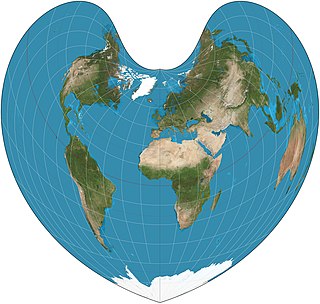
The sinusoidal projection is a pseudocylindrical equal-area map projection, sometimes called the Sanson–Flamsteed or the Mercator equal-area projection. Jean Cossin of Dieppe was one of the first mapmakers to use the sinusoidal, appearing in a world map of 1570.
The Bonne projection is a pseudoconical equal-area map projection, sometimes called a dépôt de la guerre, modified Flamsteed, or a Sylvanus projection. Although named after Rigobert Bonne (1727–1795), the projection was in use prior to his birth, in 1511 by Sylvanus, Honter in 1561, De l'Isle before 1700 and Coronelli in 1696. Both Sylvanus and Honter's usages were approximate, however, and it is not clear they intended to be the same projection.
The Universal Transverse Mercator (UTM) is a map projection system for assigning coordinates to locations on the surface of the Earth. Like the traditional method of latitude and longitude, it is a horizontal position representation, which means it ignores altitude and treats the earth surface as a perfect ellipsoid. However, it differs from global latitude/longitude in that it divides earth into 60 zones and projects each to the plane as a basis for its coordinates. Specifying a location means specifying the zone and the x, y coordinate in that plane. The projection from spheroid to a UTM zone is some parameterization of the transverse Mercator projection. The parameters vary by nation or region or mapping system.
In cartography, a Tissot's indicatrix is a mathematical contrivance presented by French mathematician Nicolas Auguste Tissot in 1859 and 1871 in order to characterize local distortions due to map projection. It is the geometry that results from projecting a circle of infinitesimal radius from a curved geometric model, such as a globe, onto a map. Tissot proved that the resulting diagram is an ellipse whose axes indicate the two principal directions along which scale is maximal and minimal at that point on the map.
The Miller cylindrical projection is a modified Mercator projection, proposed by Osborn Maitland Miller in 1942. The latitude is scaled by a factor of 4⁄5, projected according to Mercator, and then the result is multiplied by 5⁄4 to retain scale along the equator. Hence:
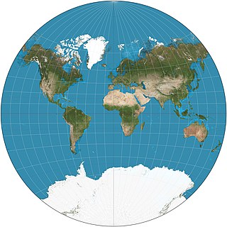
The van der Grinten projection is a compromise map projection, which means that it is neither equal-area nor conformal. Unlike perspective projections, the van der Grinten projection is an arbitrary geometric construction on the plane. Van der Grinten projects the entire Earth into a circle. It largely preserves the familiar shapes of the Mercator projection while modestly reducing Mercator's distortion. Polar regions are subject to extreme distortion. Lines of longitude converge to points at the poles.
The Aitoff projection is a modified azimuthal map projection proposed by David A. Aitoff in 1889. Based on the equatorial form of the azimuthal equidistant projection, Aitoff first halves longitudes, then projects according to the azimuthal equidistant, and then stretches the result horizontally into a 2:1 ellipse to compensate for having halved the longitudes.
The Cassini projection is a map projection first described in an approximate form by César-François Cassini de Thury in 1745. Its precise formulas were found through later analysis by Johann Georg von Soldner around 1810. It is the transverse aspect of the equirectangular projection, in that the globe is first rotated so the central meridian becomes the "equator", and then the normal equirectangular projection is applied. Considering the earth as a sphere, the projection is composed of the operations:
The Tobler hyperelliptical projection is a family of equal-area pseudocylindrical projections that may be used for world maps. Waldo R. Tobler introduced the construction in 1973 as the hyperelliptical projection, now usually known as the Tobler hyperelliptical projection.
Wagner VI is a pseudocylindrical whole Earth map projection. Like the Robinson projection, it is a compromise projection, not having any special attributes other than a pleasing, low distortion appearance. Wagner VI is equivalent to the Kavrayskiy VII horizontally elongated by a factor of ⁄. This elongation results in proper preservation of shapes near the equator but slightly more distortion overall. The aspect ratio of this projection is 2:1, as formed by the ratio of the equator to the central meridian. This matches the ratio of Earth’s equator to any meridian.
The equidistant conic projection is a conic map projection commonly used for maps of small countries as well as for larger regions such as the continental United States that are elongated east-to-west.
In the cartography of the United States, the American polyconic projection is a map projection used for maps of the United States and its regions beginning early in the 19th century. It belongs to the polyconic projection class, which consists of map projections whose parallels are non-concentric circular arcs except for the equator, which is straight. Often the American polyconic is simply called the polyconic projection.
The rectangular polyconic projection is a map projection was first mentioned in 1853 by the United States Coast Survey, where it was developed and used for portions of the U.S. exceeding about one square degree. It belongs to the polyconic projection class, which consists of map projections whose parallels are non-concentric circular arcs except for the equator, which is straight. Sometimes the rectangular polyconic is called the War Office projection due to its use by the British War Office for topographic maps. It is not used much these days, with practically all military grid systems having moved onto conformal projection systems, typically modeled on the transverse Mercator projection.
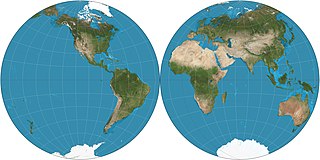
The Nicolosi globular projection is a polyconic map projection invented about the year 1,000 by the Iranian polymath al-Biruni. As a circular representation of a hemisphere, it is called globular because it evokes a globe. It can only display one hemisphere at a time and so normally appears as a "double hemispheric" presentation in world maps. The projection came into use in the Western world starting in 1660, reaching its most common use in the 19th century. As a "compromise" projection, it preserves no particular properties, instead giving a balance of distortions.
References
1 2 3 4 5 Snyder, John P. (1987). Map Projections - A Working Manual. U.S. Geological Survey Professional Paper 1395. United States Government Printing Office, Washington, D.C.This paper can be downloaded from USGS pages. It gives full details of most projections, together with introductory sections, but it does not derive any of the projections from first principles. Derivation of all the formulae for the Mercator projections may be found in The Mercator Projections.
1 2 3 4 Flattening the Earth: Two Thousand Years of Map Projections, John P. Snyder, 1993, pp. 5-8, ISBN0-226-76747-7. This is a survey of virtually all known projections from antiquity to 1993.
1 2 Selin, Helaine (2008). Encyclopaedia of the History of Science, Technology, and Medicine in Non-Western Cultures. Springer (published March 17, 2008). p.567. ISBN978-1402049606.
This page is based on this Wikipedia article Text is available under the CC BY-SA 4.0 license; additional terms may apply. Images, videos and audio are available under their respective licenses.