See also
This article includes a list of general references, but it remains largely unverified because it lacks sufficient corresponding inline citations .(September 2010) |
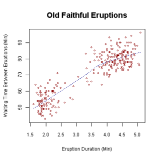
In statistics, several scatterplot smoothing methods are available to fit a function through the points of a scatterplot to best represent the relationship between the variables.
Scatterplots may be smoothed by fitting a line to the data points in a diagram. This line attempts to display the non-random component of the association between the variables in a 2D scatter plot. Smoothing attempts to separate the non-random behaviour in the data from the random fluctuations, removing or reducing these fluctuations, and allows prediction of the response based value of the explanatory variable. [1] [2]
Smoothing is normally accomplished by using any one of the techniques mentioned below.
The smoothing curve is chosen so as to provide the best fit in some sense, often defined as the fit that results in the minimum sum of the squared errors (a least squares criterion).
This article includes a list of general references, but it remains largely unverified because it lacks sufficient corresponding inline citations .(September 2010) |

In mathematics, a time series is a series of data points indexed in time order. Most commonly, a time series is a sequence taken at successive equally spaced points in time. Thus it is a sequence of discrete-time data. Examples of time series are heights of ocean tides, counts of sunspots, and the daily closing value of the Dow Jones Industrial Average.

A scatter plot is a type of plot or mathematical diagram using Cartesian coordinates to display values for typically two variables for a set of data. If the points are coded (color/shape/size), one additional variable can be displayed. The data are displayed as a collection of points, each having the value of one variable determining the position on the horizontal axis and the value of the other variable determining the position on the vertical axis.
In statistics and optimization, errors and residuals are two closely related and easily confused measures of the deviation of an observed value of an element of a statistical sample from its "theoretical value". The error of an observed value is the deviation of the observed value from the (unobservable) true value of a quantity of interest, and the residual of an observed value is the difference between the observed value and the estimated value of the quantity of interest. The distinction is most important in regression analysis, where the concepts are sometimes called the regression errors and regression residuals and where they lead to the concept of studentized residuals.

Curve fitting is the process of constructing a curve, or mathematical function, that has the best fit to a series of data points, possibly subject to constraints. Curve fitting can involve either interpolation, where an exact fit to the data is required, or smoothing, in which a "smooth" function is constructed that approximately fits the data. A related topic is regression analysis, which focuses more on questions of statistical inference such as how much uncertainty is present in a curve that is fit to data observed with random errors. Fitted curves can be used as an aid for data visualization, to infer values of a function where no data are available, and to summarize the relationships among two or more variables. Extrapolation refers to the use of a fitted curve beyond the range of the observed data, and is subject to a degree of uncertainty since it may reflect the method used to construct the curve as much as it reflects the observed data.
In statistics, the number of degrees of freedom is the number of values in the final calculation of a statistic that are free to vary.
In statistics, a generalized additive model (GAM) is a generalized linear model in which the linear response variable depends linearly on unknown smooth functions of some predictor variables, and interest focuses on inference about these smooth functions.

Genstat is a statistical software package with data analysis capabilities, particularly in the field of agriculture.

Local regression or local polynomial regression, also known as moving regression, is a generalization of the moving average and polynomial regression. Its most common methods, initially developed for scatterplot smoothing, are LOESS and LOWESS, both pronounced. They are two strongly related non-parametric regression methods that combine multiple regression models in a k-nearest-neighbor-based meta-model. In some fields, LOESS is known and commonly referred to as Savitzky–Golay filter.
Nonparametric regression is a category of regression analysis in which the predictor does not take a predetermined form but is constructed according to information derived from the data. That is, no parametric form is assumed for the relationship between predictors and dependent variable. Nonparametric regression requires larger sample sizes than regression based on parametric models because the data must supply the model structure as well as the model estimates.
In statistics, regression validation is the process of deciding whether the numerical results quantifying hypothesized relationships between variables, obtained from regression analysis, are acceptable as descriptions of the data. The validation process can involve analyzing the goodness of fit of the regression, analyzing whether the regression residuals are random, and checking whether the model's predictive performance deteriorates substantially when applied to data that were not used in model estimation.
In statistics, multivariate adaptive regression splines (MARS) is a form of regression analysis introduced by Jerome H. Friedman in 1991. It is a non-parametric regression technique and can be seen as an extension of linear models that automatically models nonlinearities and interactions between variables.
In applied statistics, a partial regression plot attempts to show the effect of adding another variable to a model that already has one or more independent variables. Partial regression plots are also referred to as added variable plots, adjusted variable plots, and individual coefficient plots.
A plot is a graphical technique for representing a data set, usually as a graph showing the relationship between two or more variables. The plot can be drawn by hand or by a computer. In the past, sometimes mechanical or electronic plotters were used. Graphs are a visual representation of the relationship between variables, which are very useful for humans who can then quickly derive an understanding which may not have come from lists of values. Given a scale or ruler, graphs can also be used to read off the value of an unknown variable plotted as a function of a known one, but this can also be done with data presented in tabular form. Graphs of functions are used in mathematics, sciences, engineering, technology, finance, and other areas.
In statistics, polynomial regression is a form of regression analysis in which the relationship between the independent variable x and the dependent variable y is modelled as an nth degree polynomial in x. Polynomial regression fits a nonlinear relationship between the value of x and the corresponding conditional mean of y, denoted E(y |x). Although polynomial regression fits a nonlinear model to the data, as a statistical estimation problem it is linear, in the sense that the regression function E(y | x) is linear in the unknown parameters that are estimated from the data. For this reason, polynomial regression is considered to be a special case of multiple linear regression.
In statistics, bivariate data is data on each of two variables, where each value of one of the variables is paired with a value of the other variable. Typically it would be of interest to investigate the possible association between the two variables. The association can be studied via a tabular or graphical display, or via sample statistics which might be used for inference. The method used to investigate the association would depend on the level of measurement of the variable. This association that involves exactly two variables can be termed a bivariate correlation, or bivariate association.
The following outline is provided as an overview of and topical guide to regression analysis:
In statistics, projection pursuit regression (PPR) is a statistical model developed by Jerome H. Friedman and Werner Stuetzle which is an extension of additive models. This model adapts the additive models in that it first projects the data matrix of explanatory variables in the optimal direction before applying smoothing functions to these explanatory variables.
Linear least squares (LLS) is the least squares approximation of linear functions to data. It is a set of formulations for solving statistical problems involved in linear regression, including variants for ordinary (unweighted), weighted, and generalized (correlated) residuals. Numerical methods for linear least squares include inverting the matrix of the normal equations and orthogonal decomposition methods.
The Hosmer–Lemeshow test is a statistical test for goodness of fit for logistic regression models. It is used frequently in risk prediction models. The test assesses whether or not the observed event rates match expected event rates in subgroups of the model population. The Hosmer–Lemeshow test specifically identifies subgroups as the deciles of fitted risk values. Models for which expected and observed event rates in subgroups are similar are called well calibrated.