Related Research Articles
In statistics, an estimator is a rule for calculating an estimate of a given quantity based on observed data: thus the rule, the quantity of interest and its result are distinguished. For example, the sample mean is a commonly used estimator of the population mean.
The following outline is provided as an overview of and topical guide to statistics:
In statistics, point estimation involves the use of sample data to calculate a single value which is to serve as a "best guess" or "best estimate" of an unknown population parameter. More formally, it is the application of a point estimator to the data to obtain a point estimate.
In statistics, the mean squared error (MSE) or mean squared deviation (MSD) of an estimator measures the average of the squares of the errors—that is, the average squared difference between the estimated values and the actual value. MSE is a risk function, corresponding to the expected value of the squared error loss. The fact that MSE is almost always strictly positive is because of randomness or because the estimator does not account for information that could produce a more accurate estimate. In machine learning, specifically empirical risk minimization, MSE may refer to the empirical risk, as an estimate of the true MSE.
In statistics and optimization, errors and residuals are two closely related and easily confused measures of the deviation of an observed value of an element of a statistical sample from its "true value". The error of an observation is the deviation of the observed value from the true value of a quantity of interest. The residual is the difference between the observed value and the estimated value of the quantity of interest. The distinction is most important in regression analysis, where the concepts are sometimes called the regression errors and regression residuals and where they lead to the concept of studentized residuals. In econometrics, "errors" are also called disturbances.
Ridge regression is a method of estimating the coefficients of multiple-regression models in scenarios where the independent variables are highly correlated. It has been used in many fields including econometrics, chemistry, and engineering. Also known as Tikhonov regularization, named for Andrey Tikhonov, it is a method of regularization of ill-posed problems. It is particularly useful to mitigate the problem of multicollinearity in linear regression, which commonly occurs in models with large numbers of parameters. In general, the method provides improved efficiency in parameter estimation problems in exchange for a tolerable amount of bias.
In statistics, sometimes the covariance matrix of a multivariate random variable is not known but has to be estimated. Estimation of covariance matrices then deals with the question of how to approximate the actual covariance matrix on the basis of a sample from the multivariate distribution. Simple cases, where observations are complete, can be dealt with by using the sample covariance matrix. The sample covariance matrix (SCM) is an unbiased and efficient estimator of the covariance matrix if the space of covariance matrices is viewed as an extrinsic convex cone in Rp×p; however, measured using the intrinsic geometry of positive-definite matrices, the SCM is a biased and inefficient estimator. In addition, if the random variable has a normal distribution, the sample covariance matrix has a Wishart distribution and a slightly differently scaled version of it is the maximum likelihood estimate. Cases involving missing data, heteroscedasticity, or autocorrelated residuals require deeper considerations. Another issue is the robustness to outliers, to which sample covariance matrices are highly sensitive.

In statistics, the coefficient of determination, denoted R2 or r2 and pronounced "R squared", is the proportion of the variation in the dependent variable that is predictable from the independent variable(s).
In statistics, ordinary least squares (OLS) is a type of linear least squares method for choosing the unknown parameters in a linear regression model by the principle of least squares: minimizing the sum of the squares of the differences between the observed dependent variable in the input dataset and the output of the (linear) function of the independent variable.
In statistics, resampling is the creation of new samples based on one observed sample. Resampling methods are:
- Permutation tests
- Bootstrapping
- Cross validation
The James–Stein estimator is a biased estimator of the mean, , of (possibly) correlated Gaussian distributed random variables with unknown means .
In statistics, the bias of an estimator is the difference between this estimator's expected value and the true value of the parameter being estimated. An estimator or decision rule with zero bias is called unbiased. In statistics, "bias" is an objective property of an estimator. Bias is a distinct concept from consistency: consistent estimators converge in probability to the true value of the parameter, but may be biased or unbiased; see bias versus consistency for more.
In statistics, Bessel's correction is the use of n − 1 instead of n in the formula for the sample variance and sample standard deviation, where n is the number of observations in a sample. This method corrects the bias in the estimation of the population variance. It also partially corrects the bias in the estimation of the population standard deviation. However, the correction often increases the mean squared error in these estimations. This technique is named after Friedrich Bessel.
In statistics, principal component regression (PCR) is a regression analysis technique that is based on principal component analysis (PCA). More specifically, PCR is used for estimating the unknown regression coefficients in a standard linear regression model.
In statistical theory, the field of high-dimensional statistics studies data whose dimension is larger than typically considered in classical multivariate analysis. The area arose owing to the emergence of many modern data sets in which the dimension of the data vectors may be comparable to, or even larger than, the sample size, so that justification for the use of traditional techniques, often based on asymptotic arguments with the dimension held fixed as the sample size increased, was lacking.
In statistics, efficiency is a measure of quality of an estimator, of an experimental design, or of a hypothesis testing procedure. Essentially, a more efficient estimator needs fewer input data or observations than a less efficient one to achieve the Cramér–Rao bound. An efficient estimator is characterized by having the smallest possible variance, indicating that there is a small deviance between the estimated value and the "true" value in the L2 norm sense.

In statistics and machine learning, the bias–variance tradeoff describes the relationship between a model's complexity, the accuracy of its predictions, and how well it can make predictions on previously unseen data that were not used to train the model. In general, as we increase the number of tunable parameters in a model, it becomes more flexible, and can better fit a training data set. It is said to have lower error, or bias. However, for more flexible models, there will tend to be greater variance to the model fit each time we take a set of samples to create a new training data set. It is said that there is greater variance in the model's estimated parameters.
In statistics, linear regression is a linear approach for modelling the relationship between a scalar response and one or more explanatory variables. The case of one explanatory variable is called simple linear regression; for more than one, the process is called multiple linear regression. This term is distinct from multivariate linear regression, where multiple correlated dependent variables are predicted, rather than a single scalar variable.
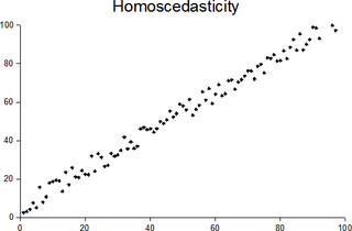
In statistics, a sequence of random variables is homoscedastic if all its random variables have the same finite variance; this is also known as homogeneity of variance. The complementary notion is called heteroscedasticity, also known as heterogeneity of variance. The spellings homoskedasticity and heteroskedasticity are also frequently used. Assuming a variable is homoscedastic when in reality it is heteroscedastic results in unbiased but inefficient point estimates and in biased estimates of standard errors, and may result in overestimating the goodness of fit as measured by the Pearson coefficient.
References
- ↑ Everitt B.S. (2002) Cambridge Dictionary of Statistics (2nd Edition), CUP. ISBN 0-521-81099-X
- ↑ Copas, J.B. (1983). "Regression, Prediction and Shrinkage". Journal of the Royal Statistical Society, Series B . 45 (3): 311–354. JSTOR 2345402. MR 0737642.
- ↑ Copas, J.B. (1993). "The shrinkage of point scoring methods". Journal of the Royal Statistical Society, Series C . 42 (2): 315–331. JSTOR 2986235.
- ↑ Hausser, Jean; Strimmer (2009). "Entropy Inference and the James-Stein Estimator, with Application to Nonlinear Gene Association Networks" (PDF). Journal of Machine Learning Research. 10: 1469–1484. Retrieved 2013-03-23.
| | This statistics-related article is a stub. You can help Wikipedia by expanding it. |