
In vector calculus, divergence is a vector operator that operates on a vector field, producing a scalar field giving the quantity of the vector field's source at each point. More technically, the divergence represents the volume density of the outward flux of a vector field from an infinitesimal volume around a given point.
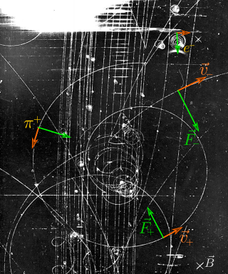
In physics, the Lorentz force is the combination of electric and magnetic force on a point charge due to electromagnetic fields. A particle of charge q moving with a velocity v in an electric field E and a magnetic field B experiences a force of

In mathematics and physics, Laplace's equation is a second-order partial differential equation named after Pierre-Simon Laplace, who first studied its properties. This is often written as

The Navier–Stokes equations are partial differential equations which describe the motion of viscous fluid substances, named after French engineer and physicist Claude-Louis Navier and Irish physicist and mathematician George Gabriel Stokes. They were developed over several decades of progressively building the theories, from 1822 (Navier) to 1842–1850 (Stokes).
In vector calculus, the divergence theorem, also known as Gauss's theorem or Ostrogradsky's theorem, is a theorem which relates the flux of a vector field through a closed surface to the divergence of the field in the volume enclosed.
In mathematics, the Laplace operator or Laplacian is a differential operator given by the divergence of the gradient of a scalar function on Euclidean space. It is usually denoted by the symbols , (where is the nabla operator), or . In a Cartesian coordinate system, the Laplacian is given by the sum of second partial derivatives of the function with respect to each independent variable. In other coordinate systems, such as cylindrical and spherical coordinates, the Laplacian also has a useful form. Informally, the Laplacian Δf (p) of a function f at a point p measures by how much the average value of f over small spheres or balls centered at p deviates from f (p).
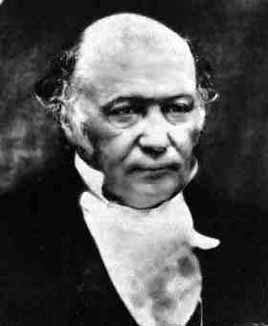
Hamiltonian mechanics emerged in 1833 as a reformulation of Lagrangian mechanics. Introduced by Sir William Rowan Hamilton, Hamiltonian mechanics replaces (generalized) velocities used in Lagrangian mechanics with (generalized) momenta. Both theories provide interpretations of classical mechanics and describe the same physical phenomena.
In mathematics, the covariant derivative is a way of specifying a derivative along tangent vectors of a manifold. Alternatively, the covariant derivative is a way of introducing and working with a connection on a manifold by means of a differential operator, to be contrasted with the approach given by a principal connection on the frame bundle – see affine connection. In the special case of a manifold isometrically embedded into a higher-dimensional Euclidean space, the covariant derivative can be viewed as the orthogonal projection of the Euclidean directional derivative onto the manifold's tangent space. In this case the Euclidean derivative is broken into two parts, the extrinsic normal component and the intrinsic covariant derivative component.
This is a list of some vector calculus formulae for working with common curvilinear coordinate systems.
In mathematics and physics, the Christoffel symbols are an array of numbers describing a metric connection. The metric connection is a specialization of the affine connection to surfaces or other manifolds endowed with a metric, allowing distances to be measured on that surface. In differential geometry, an affine connection can be defined without reference to a metric, and many additional concepts follow: parallel transport, covariant derivatives, geodesics, etc. also do not require the concept of a metric. However, when a metric is available, these concepts can be directly tied to the "shape" of the manifold itself; that shape is determined by how the tangent space is attached to the cotangent space by the metric tensor. Abstractly, one would say that the manifold has an associated (orthonormal) frame bundle, with each "frame" being a possible choice of a coordinate frame. An invariant metric implies that the structure group of the frame bundle is the orthogonal group O(p, q). As a result, such a manifold is necessarily a (pseudo-)Riemannian manifold. The Christoffel symbols provide a concrete representation of the connection of (pseudo-)Riemannian geometry in terms of coordinates on the manifold. Additional concepts, such as parallel transport, geodesics, etc. can then be expressed in terms of Christoffel symbols.
In differential geometry, the four-gradient is the four-vector analogue of the gradient from vector calculus.
The electromagnetic wave equation is a second-order partial differential equation that describes the propagation of electromagnetic waves through a medium or in a vacuum. It is a three-dimensional form of the wave equation. The homogeneous form of the equation, written in terms of either the electric field E or the magnetic field B, takes the form:
The following are important identities involving derivatives and integrals in vector calculus.
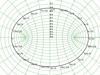
In geometry, the elliptic coordinate system is a two-dimensional orthogonal coordinate system in which the coordinate lines are confocal ellipses and hyperbolae. The two foci and are generally taken to be fixed at and , respectively, on the -axis of the Cartesian coordinate system.

Elliptic cylindrical coordinates are a three-dimensional orthogonal coordinate system that results from projecting the two-dimensional elliptic coordinate system in the perpendicular -direction. Hence, the coordinate surfaces are prisms of confocal ellipses and hyperbolae. The two foci and are generally taken to be fixed at and , respectively, on the -axis of the Cartesian coordinate system.
In physics, the Green's function for Laplace's equation in three variables is used to describe the response of a particular type of physical system to a point source. In particular, this Green's function arises in systems that can be described by Poisson's equation, a partial differential equation (PDE) of the form
In mathematics, vector spherical harmonics (VSH) are an extension of the scalar spherical harmonics for use with vector fields. The components of the VSH are complex-valued functions expressed in the spherical coordinate basis vectors.
In fluid dynamics, the Oseen equations describe the flow of a viscous and incompressible fluid at small Reynolds numbers, as formulated by Carl Wilhelm Oseen in 1910. Oseen flow is an improved description of these flows, as compared to Stokes flow, with the (partial) inclusion of convective acceleration.
Curvilinear coordinates can be formulated in tensor calculus, with important applications in physics and engineering, particularly for describing transportation of physical quantities and deformation of matter in fluid mechanics and continuum mechanics.
In theoretical physics, Hamiltonian field theory is the field-theoretic analogue to classical Hamiltonian mechanics. It is a formalism in classical field theory alongside Lagrangian field theory. It also has applications in quantum field theory.


