Stochastic dominance

For other uses, see Dominance.

Stochastic dominance is a partial order between random variables. ^{[1] [2]} It is a form of stochastic ordering. The concept arises in decision theory and decision analysis in situations where one gamble (a probability distribution over possible outcomes, also known as prospects) can be ranked as superior to another gamble for a broad class of decision-makers. It is based on shared preferences regarding sets of possible outcomes and their associated probabilities. Only limited knowledge of preferences is required for determining dominance. Risk aversion is a factor only in second order stochastic dominance.

Stochastic dominance does not give a total order, but rather only a partial order: for some pairs of gambles, neither one stochastically dominates the other, since different members of the broad class of decision-makers will differ regarding which gamble is preferable without them generally being considered to be equally attractive.

Throughout the article, ${\displaystyle \rho ,\nu }$ stand for probability distributions on ${\displaystyle \mathbb {R} }$, while ${\displaystyle A,B,X,Y,Z}$ stand for particular random variables on ${\displaystyle \mathbb {R} }$. The notation ${\displaystyle X\sim \rho }$ means that ${\displaystyle X}$ has distribution ${\displaystyle \rho }$.

There are a sequence of stochastic dominance orderings, from first ${\displaystyle \succeq _{1}}$, to second ${\displaystyle \succeq _{2}}$, to higher orders ${\displaystyle \succeq _{n}}$. The sequence is increasingly more inclusive. That is, if ${\displaystyle \rho \succeq _{n}\nu }$, then ${\displaystyle \rho \succeq _{k}\nu }$ for all ${\displaystyle k\leq n}$. Further, there exists ${\displaystyle \rho ,\nu }$ such that ${\displaystyle \rho \succeq _{n+1}\nu }$ but not ${\displaystyle \rho \succeq _{n}\nu }$^{[ contradictory ]}.

Stochastic dominance could trace back to (Blackwell, 1953), ^[3] but it was not developed until 1969–1970. ^[4]

Statewise dominance (Zeroth-Order)

The simplest case of stochastic dominance is statewise dominance (also known as state-by-state dominance), defined as follows:

Random variable A is statewise dominant over random variable B if A gives at least as good a result in every state (every possible set of outcomes), and a strictly better result in at least one state.

For example, if a dollar is added to one or more prizes in a lottery, the new lottery statewise dominates the old one because it yields a better payout regardless of the specific numbers realized by the lottery. Similarly, if a risk insurance policy has a lower premium and a better coverage than another policy, then with or without damage, the outcome is better. Anyone who prefers more to less (in the standard terminology, anyone who has monotonically increasing preferences) will always prefer a statewise dominant gamble.

First-order

${\displaystyle F_{B\sim N(0,1)}(x)\geq F_{A\sim N(0.75,1)}(x)\forall x}$${\displaystyle \implies B(black)\leq A(red)}$

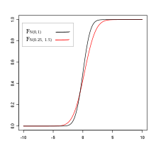
${\displaystyle F_{X\sim N(0,1)}}$ und ${\displaystyle F_{Y\sim N(0.25,1.5)}}$, X and Y are not compareable through first-order stochastic dominance.

Statewise dominance implies first-order stochastic dominance (FSD), ^[5] which is defined as:

Random variable A has first-order stochastic dominance over random variable B if for any outcome x, A gives at least as high a probability of receiving at least x as does B, and for some x, A gives a higher probability of receiving at least x. In notation form, ${\displaystyle P[A\geq x]\geq P[B\geq x]}$ for all x, and for some x, ${\displaystyle P[A\geq x]>P[B\geq x]}$.

In terms of the cumulative distribution functions of the two random variables, A dominating B means that ${\displaystyle F_{A}(x)\leq F_{B}(x)}$ for all x, with strict inequality at some x.

In the case of non-intersecting^{[ clarification needed ]} distribution functions, the Wilcoxon rank-sum test tests for first-order stochastic dominance. ^[6]

Equivalent definitions

Let ${\displaystyle \rho ,\nu }$ be two probability distributions on ${\displaystyle \mathbb {R} }$, such that ${\displaystyle \mathbb {E} _{X\sim \rho }[|X|],\mathbb {E} _{X\sim \nu }[|X|]}$ are both finite, then the following conditions are equivalent, thus they may all serve as the definition of first-order stochastic dominance: ^[7]

• For any ${\displaystyle u:\mathbb {R} \to \mathbb {R} }$ that is non-decreasing, ${\displaystyle \mathbb {E} _{X\sim \rho }[u(X)]\geq \mathbb {E} _{X\sim \nu }[u(X)]}$

• ${\displaystyle F_{\rho }(t)\leq F_{\nu }(t),\quad \forall t\in \mathbb {R} .}$
• There exists two random variables ${\displaystyle X\sim \rho ,Y\sim \nu }$, such that ${\displaystyle X=Y+\delta }$, where ${\displaystyle \delta \geq 0}$.

The first definition states that a gamble ${\displaystyle \rho }$ first-order stochastically dominates gamble ${\displaystyle \nu }$ if and only if every expected utility maximizer with an increasing utility function prefers gamble ${\displaystyle \rho }$ over gamble ${\displaystyle \nu }$.

The third definition states that we can construct a pair of gambles ${\displaystyle X,Y}$ with distributions ${\displaystyle \rho ,\nu }$, such that gamble ${\displaystyle X}$ always pays at least as much as gamble ${\displaystyle Y}$. More concretely, construct first a uniformly distributed ${\displaystyle Z\sim \mathrm {Uniform} (0,1)}$, then use the inverse transform sampling to get ${\displaystyle X=F_{X}^{-1}(Z),Y=F_{Y}^{-1}(Z)}$, then ${\displaystyle X\geq Y}$ for any ${\displaystyle Z}$.

Pictorially, the second and third definition are equivalent, because we can go from the graphed density function of A to that of B both by pushing it upwards and pushing it leftwards.

Extended example

Consider three gambles over a single toss of a fair six-sided die:

${\displaystyle {\begin{array}{rcccccc}{\text{State (die result)}}&1&2&3&4&5&6\\\hline {\text{gamble A wins }}\$&1&1&2&2&2&2\\{\text{gamble B wins }}\$&1&1&1&2&2&2\\{\text{gamble C wins }}\$&3&3&3&1&1&1\\\hline \end{array}}}$

Gamble A statewise dominates gamble B because A gives at least as good a yield in all possible states (outcomes of the die roll) and gives a strictly better yield in one of them (state 3). Since A statewise dominates B, it also first-order dominates B.

Gamble C does not statewise dominate B because B gives a better yield in states 4 through 6, but C first-order stochastically dominates B because Pr(B ≥ 1) = Pr(C ≥ 1) = 1, Pr(B ≥ 2) = Pr(C ≥ 2) = 3/6, and Pr(B ≥ 3) = 0 while Pr(C ≥ 3) = 3/6 > Pr(B ≥ 3).

Gambles A and C cannot be ordered relative to each other on the basis of first-order stochastic dominance because Pr(A ≥ 2) = 4/6 > Pr(C ≥ 2) = 3/6 while on the other hand Pr(C ≥ 3) = 3/6 > Pr(A ≥ 3) = 0.

In general, although when one gamble first-order stochastically dominates a second gamble, the expected value of the payoff under the first will be greater than the expected value of the payoff under the second, the converse is not true: one cannot order lotteries with regard to stochastic dominance simply by comparing the means of their probability distributions. For instance, in the above example C has a higher mean (2) than does A (5/3), yet C does not first-order dominate A.

Second-order

The other commonly used type of stochastic dominance is second-order stochastic dominance. ^{[1] [8] [9]} Roughly speaking, for two gambles ${\displaystyle \rho }$ and ${\displaystyle \nu }$, gamble ${\displaystyle \rho }$ has second-order stochastic dominance over gamble ${\displaystyle \nu }$ if the former is more predictable (i.e. involves less risk) and has at least as high a mean. All risk-averse expected-utility maximizers (that is, those with increasing and concave utility functions) prefer a second-order stochastically dominant gamble to a dominated one. Second-order dominance describes the shared preferences of a smaller class of decision-makers (those for whom more is better and who are averse to risk, rather than all those for whom more is better) than does first-order dominance.

In terms of cumulative distribution functions ${\displaystyle F_{\rho }}$ and ${\displaystyle F_{\nu }}$, ${\displaystyle \rho }$ is second-order stochastically dominant over ${\displaystyle \nu }$ if and only if ${\displaystyle \int _{-\infty }^{x}[F_{\nu }(t)-F_{\rho }(t)]\,dt\geq 0}$ for all ${\displaystyle x}$, with strict inequality at some ${\displaystyle x}$. Equivalently, ${\displaystyle \rho }$ dominates ${\displaystyle \nu }$ in the second order if and only if ${\displaystyle \mathbb {E} _{X\sim \rho }[u(X)]\geq \mathbb {E} _{X\sim \nu }[u(X)]}$ for all nondecreasing and concave utility functions ${\displaystyle u(x)}$.

Second-order stochastic dominance can also be expressed as follows: Gamble ${\displaystyle \rho }$ second-order stochastically dominates ${\displaystyle \nu }$ if and only if there exist some gambles ${\displaystyle y}$ and ${\displaystyle z}$ such that ${\displaystyle x_{\nu }{\overset {d}{=}}(x_{\rho }+y+z)}$, with ${\displaystyle y}$ always less than or equal to zero, and with ${\displaystyle \mathbb {E} (z\mid x_{\rho }+y)=0}$ for all values of ${\displaystyle x_{\rho }+y}$. Here the introduction of random variable ${\displaystyle y}$ makes ${\displaystyle \nu }$ first-order stochastically dominated by ${\displaystyle \rho }$ (making ${\displaystyle \nu }$ disliked by those with an increasing utility function), and the introduction of random variable ${\displaystyle z}$ introduces a mean-preserving spread in ${\displaystyle \nu }$ which is disliked by those with concave utility. Note that if ${\displaystyle \rho }$ and ${\displaystyle \nu }$ have the same mean (so that the random variable ${\displaystyle y}$ degenerates to the fixed number 0), then ${\displaystyle \nu }$ is a mean-preserving spread of ${\displaystyle \rho }$.

Equivalent definitions

Let ${\displaystyle \rho ,\nu }$ be two probability distributions on ${\displaystyle \mathbb {R} }$, such that ${\displaystyle \mathbb {E} _{X\sim \rho }[|X|],\mathbb {E} _{X\sim \nu }[|X|]}$ are both finite, then the following conditions are equivalent, thus they may all serve as the definition of second-order stochastic dominance: ^[7]

• For any ${\displaystyle u:\mathbb {R} \to \mathbb {R} }$ that is non-decreasing, and (not necessarily strictly) concave,${\displaystyle \mathbb {E} _{X\sim \rho }[u(X)]\geq \mathbb {E} _{X\sim \nu }[u(X)]}$

• ${\displaystyle \int _{-\infty }^{t}F_{\rho }(x)dx\leq \int _{-\infty }^{t}F_{\nu }(x)dx,\quad \forall t\in \mathbb {R} .}$
• There exists two random variables ${\displaystyle X\sim \rho ,Y\sim \nu }$, such that ${\displaystyle Y=X-\delta +\epsilon }$, where ${\displaystyle \delta \geq 0}$ and ${\displaystyle \mathbb {E} [\epsilon |X-\delta ]=0}$.

These are analogous with the equivalent definitions of first-order stochastic dominance, given above.

Sufficient conditions

• First-order stochastic dominance of A over B is a sufficient condition for second-order dominance of A over B.
• If B is a mean-preserving spread of A, then A second-order stochastically dominates B.

Necessary conditions

• ${\displaystyle \mathbb {E} _{\rho }(x)\geq \mathbb {E} _{\nu }(x)}$ is a necessary condition for A to second-order stochastically dominate B.
• ${\displaystyle \min _{\rho }(x)\geq \min _{\nu }(x)}$ is a necessary condition for A to second-order dominate B. The condition implies that the left tail of ${\displaystyle F_{\nu }}$ must be thicker than the left tail of ${\displaystyle F_{\rho }}$.

Third-order

Let ${\displaystyle F_{\rho }}$ and ${\displaystyle F_{\nu }}$ be the cumulative distribution functions of two distinct investments ${\displaystyle \rho }$ and ${\displaystyle \nu }$. ${\displaystyle \rho }$ dominates ${\displaystyle \nu }$ in the third order if and only if both

• ${\displaystyle \int _{-\infty }^{x}\left(\int _{-\infty }^{z}[F_{\nu }(t)-F_{\rho }(t)]\,dt\right)dz\geq 0{\text{ for all }}x,}$
• ${\displaystyle \mathbb {E} _{\rho }(x)\geq \mathbb {E} _{\nu }(x)}$.

Equivalently, ${\displaystyle \rho }$ dominates ${\displaystyle \nu }$ in the third order if and only if ${\displaystyle \mathbb {E} _{\rho }U(x)\geq \mathbb {E} _{\nu }U(x)}$ for all ${\displaystyle U\in D_{3}}$.

The set ${\displaystyle D_{3}}$ has two equivalent definitions:

• the set of nondecreasing, concave utility functions that are positively skewed (that is, have a nonnegative third derivative throughout). ^[10]
• the set of nondecreasing, concave utility functions, such that for any random variable ${\displaystyle Z}$, the risk-premium function ${\displaystyle \pi _{u}(x,Z)}$ is a monotonically nonincreasing function of ${\displaystyle x}$. ^[11]

Here, ${\displaystyle \pi _{u}(x,Z)}$ is defined as the solution to the problem

$${\displaystyle u(x+\mathbb {E} [Z]-\pi )=\mathbb {E} [u(x+Z)].}$$

See more details at risk premium page.

Sufficient condition

• Second-order dominance is a sufficient condition.

Necessary conditions^{[ citation needed ]}

• ${\displaystyle \mathbb {E} _{\rho }(\log(x))\geq \mathbb {E} _{\nu }(\log(x))}$ is a necessary condition. The condition implies that the geometric mean of ${\displaystyle \rho }$ must be greater than or equal to the geometric mean of ${\displaystyle \nu }$.
• ${\displaystyle \min _{\rho }(x)\geq \min _{\nu }(x)}$ is a necessary condition. The condition implies that the left tail of ${\displaystyle F_{\nu }}$ must be thicker than the left tail of ${\displaystyle F_{\rho }}$.

Higher-order

Higher orders of stochastic dominance have also been analyzed, as have generalizations of the dual relationship between stochastic dominance orderings and classes of preference functions. ^[12] Arguably the most powerful dominance criterion relies on the accepted economic assumption of decreasing absolute risk aversion. ^{[13] [14]} This involves several analytical challenges and a research effort is on its way to address those. ^[15]

Formally, the n-th-order stochastic dominance is defined as ^[16]

• For any probability distribution ${\displaystyle \rho }$ on ${\displaystyle [0,\infty )}$, define the functions inductively:

$${\displaystyle F_{\rho }^{1}(t)=F_{\rho }(t),\quad F_{\rho }^{2}(t)=\int _{0}^{t}F_{\rho }^{1}(x)dx,\quad \cdots }$$

• For any two probability distributions ${\displaystyle \rho ,\nu }$ on ${\displaystyle [0,\infty )}$, non-strict and strict n-th-order stochastic dominance is defined as
  $${\displaystyle \rho \succeq _{n}\nu \quad {\text{ iff }}\quad F_{\rho }^{n}\leq F_{\nu }^{n}{\text{ on }}[0,\infty )}$$
  $${\displaystyle \rho \succ _{n}\nu \quad {\text{ iff }}\quad \rho \succeq _{n}\nu {\text{ and }}\rho \neq \nu }$$

These relations are transitive and increasingly more inclusive. That is, if ${\displaystyle \rho \succeq _{n}\nu }$, then ${\displaystyle \rho \succeq _{k}\nu }$ for all ${\displaystyle k\geq n}$. Further, there exists ${\displaystyle \rho ,\nu }$ such that ${\displaystyle \rho \succeq _{n+1}\nu }$ but not ${\displaystyle \rho \succeq _{n}\nu }$.

Define the n-th moment by ${\displaystyle \mu _{k}(\rho )=\mathbb {E} _{X\sim \rho }[X^{k}]=\int x^{k}dF_{\rho }(x)}$, then

Theorem — If ${\displaystyle \rho \succ _{n}\nu }$ are on ${\displaystyle [0,\infty )}$ with finite moments ${\displaystyle \mu _{k}(\rho ),\mu _{k}(\nu )}$ for all ${\displaystyle k=1,2,...,n}$, then ${\displaystyle (\mu _{1}(\rho ),...,\mu _{n}(\rho ))\succ _{n}^{*}(\mu _{1}(\nu ),\mu _{n}(\nu ))}$.

Here, the partial ordering ${\displaystyle \succ _{n}^{*}}$ is defined on ${\displaystyle \mathbb {R} ^{n}}$ by ${\displaystyle v\succ _{n}^{*}w}$ iff ${\displaystyle v\neq w}$, and, letting ${\displaystyle k}$ be the smallest such that ${\displaystyle v_{k}\neq w_{k}}$, we have ${\displaystyle (-1)^{k-1}v_{k}>(-1)^{k-1}w_{k}}$

Constraints

Stochastic dominance relations may be used as constraints in problems of mathematical optimization, in particular stochastic programming. ^{[17] [18] [19]} In a problem of maximizing a real functional ${\displaystyle f(X)}$ over random variables ${\displaystyle X}$ in a set ${\displaystyle X_{0}}$ we may additionally require that ${\displaystyle X}$ stochastically dominates a fixed random benchmark${\displaystyle B}$. In these problems, utility functions play the role of Lagrange multipliers associated with stochastic dominance constraints. Under appropriate conditions, the solution of the problem is also a (possibly local) solution of the problem to maximize ${\displaystyle f(X)+\mathbb {E} [u(X)-u(B)]}$ over ${\displaystyle X}$ in ${\displaystyle X_{0}}$, where ${\displaystyle u(x)}$ is a certain utility function. If the first order stochastic dominance constraint is employed, the utility function ${\displaystyle u(x)}$ is nondecreasing; if the second order stochastic dominance constraint is used, ${\displaystyle u(x)}$ is nondecreasing and concave. A system of linear equations can test whether a given solution if efficient for any such utility function. ^[20] Third-order stochastic dominance constraints can be dealt with using convex quadratically constrained programming (QCP). ^[21]

See also

• Modern portfolio theory
• Marginal conditional stochastic dominance
• Responsive set extension - equivalent to stochastic dominance in the context of preference relations.
• Quantum catalyst
• Ordinal Pareto efficiency
• Lexicographic dominance

References

1. Hadar, J.; Russell, W. (1969). "Rules for Ordering Uncertain Prospects". American Economic Review . 59 (1): 25–34. JSTOR   1811090.
2. Bawa, Vijay S. (1975). "Optimal Rules for Ordering Uncertain Prospects". Journal of Financial Economics. 2 (1): 95–121. doi:10.1016/0304-405X(75)90025-2.
3. Blackwell, David (June 1953). "Equivalent Comparisons of Experiments". The Annals of Mathematical Statistics. 24 (2): 265–272. doi: 10.1214/aoms/1177729032 . ISSN   0003-4851.
4. Levy, Haim (1990), Eatwell, John; Milgate, Murray; Newman, Peter (eds.), "Stochastic Dominance", Utility and Probability, London: Palgrave Macmillan UK, pp. 251–254, doi:10.1007/978-1-349-20568-4_34, ISBN   978-1-349-20568-4 , retrieved 2022-12-23
5. Quirk, J. P.; Saposnik, R. (1962). "Admissibility and Measurable Utility Functions". Review of Economic Studies . 29 (2): 140–146. doi:10.2307/2295819. JSTOR   2295819.
6. Seifert, S. (2006). Posted Price Offers in Internet Auction Markets. Deutschland: Physica-Verlag. Page 85, ISBN 9783540352686, https://books.google.de/books?id=a-ngTxeSLakC&pg=PA85
7. Mas-Colell, Andreu; Whinston, Michael Dennis; Green, Jerry R. (1995). Microeconomic theory. New York. Proposition 6.D.1. ISBN   0-19-507340-1. OCLC   32430901.
8. Hanoch, G.; Levy, H. (1969). "The Efficiency Analysis of Choices Involving Risk". Review of Economic Studies. 36 (3): 335–346. doi:10.2307/2296431. JSTOR   2296431.
9. Rothschild, M.; Stiglitz, J. E. (1970). "Increasing Risk: I. A Definition". Journal of Economic Theory . 2 (3): 225–243. doi:10.1016/0022-0531(70)90038-4.
10. Chan, Raymond H.; Clark, Ephraim; Wong, Wing-Keung (2012-11-16). "On the Third Order Stochastic Dominance for Risk-Averse and Risk-Seeking Investors". mpra.ub.uni-muenchen.de. Retrieved 2022-12-25.
11. Whitmore, G. A. (1970). "Third-Degree Stochastic Dominance". The American Economic Review. 60 (3): 457–459. ISSN   0002-8282. JSTOR   1817999.
12. Ekern, Steinar (1980). "Increasing Nth Degree Risk". Economics Letters. 6 (4): 329–333. doi:10.1016/0165-1765(80)90005-1.
13. Vickson, R.G. (1975). "Stochastic Dominance Tests for Decreasing Absolute Risk Aversion. I. Discrete Random Variables". Management Science. 21 (12): 1438–1446. doi:10.1287/mnsc.21.12.1438.
14. Vickson, R.G. (1977). "Stochastic Dominance Tests for Decreasing Absolute Risk Aversion. II. General random Variables". Management Science. 23 (5): 478–489. doi:10.1287/mnsc.23.5.478.
15. See, e.g. Post, Th.; Fang, Y.; Kopa, M. (2015). "Linear Tests for DARA Stochastic Dominance". Management Science. 61 (7): 1615–1629. doi:10.1287/mnsc.2014.1960.
16. Fishburn, Peter C. (1980-02-01). "Stochastic Dominance and Moments of Distributions". Mathematics of Operations Research . 5 (1): 94–100. doi:10.1287/moor.5.1.94. ISSN   0364-765X.
17. Dentcheva, D.; Ruszczyński, A. (2003). "Optimization with Stochastic Dominance Constraints". SIAM Journal on Optimization. 14 (2): 548–566. CiteSeerX   10.1.1.201.7815 . doi:10.1137/S1052623402420528. S2CID   12502544.
18. Kuosmanen, T (2004). "Efficient diversification according to stochastic dominance criteria". Management Science. 50 (10): 1390–1406. doi:10.1287/mnsc.1040.0284.
19. Dentcheva, D.; Ruszczyński, A. (2004). "Semi-Infinite Probabilistic Optimization: First Order Stochastic Dominance Constraints". Optimization. 53 (5–6): 583–601. doi:10.1080/02331930412331327148. S2CID   122168294.
20. Post, Th (2003). "Empirical tests for stochastic dominance efficiency". Journal of Finance. 58 (5): 1905–1932. doi:10.1111/1540-6261.00592.
21. Post, Thierry; Kopa, Milos (2016). "Portfolio Choice Based on Third-Degree Stochastic Dominance". Management Science . 63 (10): 3381–3392. doi:10.1287/mnsc.2016.2506. SSRN   2687104.