Tensor derivative (continuum mechanics)

Last updated

The derivatives of scalars, vectors, and second-order tensors with respect to second-order tensors are of considerable use in continuum mechanics. These derivatives are used in the theories of nonlinear elasticity and plasticity, particularly in the design of algorithms for numerical simulations. [1]

Contents

The directional derivative provides a systematic way of finding these derivatives. [2]

Derivatives with respect to vectors and second-order tensors

The definitions of directional derivatives for various situations are given below. It is assumed that the functions are sufficiently smooth that derivatives can be taken.

Derivatives of scalar valued functions of vectors

Let f(v) be a real valued function of the vector v. Then the derivative of f(v) with respect to v (or at v) is the vector defined through its dot product with any vector u being

for all vectors u. The above dot product yields a scalar, and if u is a unit vector gives the directional derivative of f at v, in the u direction.

Properties:

  1. If then
  2. If then
  3. If then

Derivatives of vector valued functions of vectors

Let f(v) be a vector valued function of the vector v. Then the derivative of f(v) with respect to v (or at v) is the second order tensor defined through its dot product with any vector u being

for all vectors u. The above dot product yields a vector, and if u is a unit vector gives the direction derivative of f at v, in the directional u.

Properties:

  1. If then
  2. If then
  3. If then

Derivatives of scalar valued functions of second-order tensors

Let be a real valued function of the second order tensor . Then the derivative of with respect to (or at ) in the direction is the second order tensor defined as

for all second order tensors .

Properties:

  1. If then
  2. If then
  3. If then

Derivatives of tensor valued functions of second-order tensors

Let be a second order tensor valued function of the second order tensor . Then the derivative of with respect to (or at ) in the direction is the fourth order tensor defined as

for all second order tensors .

Properties:

  1. If then
  2. If then
  3. If then
  4. If then

Gradient of a tensor field

The gradient, , of a tensor field in the direction of an arbitrary constant vector c is defined as:

The gradient of a tensor field of order n is a tensor field of order n+1.

Cartesian coordinates

If are the basis vectors in a Cartesian coordinate system, with coordinates of points denoted by (), then the gradient of the tensor field is given by

Proof

The vectors x and c can be written as and . Let y := x + αc. In that case the gradient is given by

Since the basis vectors do not vary in a Cartesian coordinate system we have the following relations for the gradients of a scalar field , a vector field v, and a second-order tensor field .

Curvilinear coordinates

If are the contravariant basis vectors in a curvilinear coordinate system, with coordinates of points denoted by (), then the gradient of the tensor field is given by (see [3] for a proof.)

From this definition we have the following relations for the gradients of a scalar field , a vector field v, and a second-order tensor field .

where the Christoffel symbol is defined using

Cylindrical polar coordinates

In cylindrical coordinates, the gradient is given by

Divergence of a tensor field

The divergence of a tensor field is defined using the recursive relation

where c is an arbitrary constant vector and v is a vector field. If is a tensor field of order n > 1 then the divergence of the field is a tensor of order n− 1.

Cartesian coordinates

In a Cartesian coordinate system we have the following relations for a vector field v and a second-order tensor field .

where tensor index notation for partial derivatives is used in the rightmost expressions. Note that

For a symmetric second-order tensor, the divergence is also often written as [4]

The above expression is sometimes used as the definition of in Cartesian component form (often also written as ). Note that such a definition is not consistent with the rest of this article (see the section on curvilinear co-ordinates).

The difference stems from whether the differentiation is performed with respect to the rows or columns of , and is conventional. This is demonstrated by an example. In a Cartesian coordinate system the second order tensor (matrix) is the gradient of a vector function .

The last equation is equivalent to the alternative definition / interpretation [4]

Curvilinear coordinates

In curvilinear coordinates, the divergences of a vector field v and a second-order tensor field are

More generally,


Cylindrical polar coordinates

In cylindrical polar coordinates

Curl of a tensor field

The curl of an order-n > 1 tensor field is also defined using the recursive relation

where c is an arbitrary constant vector and v is a vector field.

Curl of a first-order tensor (vector) field

Consider a vector field v and an arbitrary constant vector c. In index notation, the cross product is given by

where is the permutation symbol, otherwise known as the Levi-Civita symbol. Then,

Therefore,

Curl of a second-order tensor field

For a second-order tensor

Hence, using the definition of the curl of a first-order tensor field,

Therefore, we have

Identities involving the curl of a tensor field

The most commonly used identity involving the curl of a tensor field, , is

This identity holds for tensor fields of all orders. For the important case of a second-order tensor, , this identity implies that

Derivative of the determinant of a second-order tensor

The derivative of the determinant of a second order tensor is given by

In an orthonormal basis, the components of can be written as a matrix A. In that case, the right hand side corresponds the cofactors of the matrix.

Proof

Let be a second order tensor and let . Then, from the definition of the derivative of a scalar valued function of a tensor, we have

The determinant of a tensor can be expressed in the form of a characteristic equation in terms of the invariants using

Using this expansion we can write

Recall that the invariant is given by

Hence,

Invoking the arbitrariness of we then have

Derivatives of the invariants of a second-order tensor

The principal invariants of a second order tensor are

The derivatives of these three invariants with respect to are

Proof

From the derivative of the determinant we know that

For the derivatives of the other two invariants, let us go back to the characteristic equation

Using the same approach as for the determinant of a tensor, we can show that

Now the left hand side can be expanded as

Hence

or,

Expanding the right hand side and separating terms on the left hand side gives

or,

If we define and , we can write the above as

Collecting terms containing various powers of λ, we get

Then, invoking the arbitrariness of λ, we have

This implies that

Derivative of the second-order identity tensor

Let be the second order identity tensor. Then the derivative of this tensor with respect to a second order tensor is given by

This is because is independent of .

Derivative of a second-order tensor with respect to itself

Let be a second order tensor. Then

Therefore,

Here is the fourth order identity tensor. In index notation with respect to an orthonormal basis

This result implies that

where

Therefore, if the tensor is symmetric, then the derivative is also symmetric and we get

where the symmetric fourth order identity tensor is

Derivative of the inverse of a second-order tensor

Let and be two second order tensors, then

In index notation with respect to an orthonormal basis

We also have

In index notation

If the tensor is symmetric then

Proof

Recall that

Since , we can write

Using the product rule for second order tensors

we get

or,

Therefore,

Integration by parts

Domain
O
{\displaystyle \Omega }
, its boundary
G
{\displaystyle \Gamma }
and the outward unit normal
n
{\displaystyle \mathbf {n} } StressMeasures.png
Domain , its boundary and the outward unit normal

Another important operation related to tensor derivatives in continuum mechanics is integration by parts. The formula for integration by parts can be written as

where and are differentiable tensor fields of arbitrary order, is the unit outward normal to the domain over which the tensor fields are defined, represents a generalized tensor product operator, and is a generalized gradient operator. When is equal to the identity tensor, we get the divergence theorem

We can express the formula for integration by parts in Cartesian index notation as

For the special case where the tensor product operation is a contraction of one index and the gradient operation is a divergence, and both and are second order tensors, we have

In index notation,

See also

Related Research Articles

<span class="mw-page-title-main">Navier–Stokes equations</span> Equations describing the motion of viscous fluid substances

The Navier–Stokes equations are partial differential equations which describe the motion of viscous fluid substances. They were named after French engineer and physicist Claude-Louis Navier and the Irish physicist and mathematician George Gabriel Stokes. They were developed over several decades of progressively building the theories, from 1822 (Navier) to 1842–1850 (Stokes).

In continuum mechanics, the infinitesimal strain theory is a mathematical approach to the description of the deformation of a solid body in which the displacements of the material particles are assumed to be much smaller than any relevant dimension of the body; so that its geometry and the constitutive properties of the material at each point of space can be assumed to be unchanged by the deformation.

In fluid dynamics, Stokes' law is an empirical law for the frictional force – also called drag force – exerted on spherical objects with very small Reynolds numbers in a viscous fluid. It was derived by George Gabriel Stokes in 1851 by solving the Stokes flow limit for small Reynolds numbers of the Navier–Stokes equations.

<span class="mw-page-title-main">Four-vector</span> 4-dimensional vector in relativity

In special relativity, a four-vector is an object with four components, which transform in a specific way under Lorentz transformations. Specifically, a four-vector is an element of a four-dimensional vector space considered as a representation space of the standard representation of the Lorentz group, the representation. It differs from a Euclidean vector in how its magnitude is determined. The transformations that preserve this magnitude are the Lorentz transformations, which include spatial rotations and boosts.

Linear elasticity is a mathematical model of how solid objects deform and become internally stressed due to prescribed loading conditions. It is a simplification of the more general nonlinear theory of elasticity and a branch of continuum mechanics.

A directional derivative is a concept in multivariable calculus that measures the rate at which a function changes in a particular direction at a given point.

<span class="mw-page-title-main">Curvilinear coordinates</span> Coordinate system whose directions vary in space

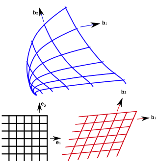
In geometry, curvilinear coordinates are a coordinate system for Euclidean space in which the coordinate lines may be curved. These coordinates may be derived from a set of Cartesian coordinates by using a transformation that is locally invertible at each point. This means that one can convert a point given in a Cartesian coordinate system to its curvilinear coordinates and back. The name curvilinear coordinates, coined by the French mathematician Lamé, derives from the fact that the coordinate surfaces of the curvilinear systems are curved.

<span class="mw-page-title-main">Cartesian tensor</span>

In geometry and linear algebra, a Cartesian tensor uses an orthonormal basis to represent a tensor in a Euclidean space in the form of components. Converting a tensor's components from one such basis to another is done through an orthogonal transformation.

In continuum mechanics, the finite strain theory—also called large strain theory, or large deformation theory—deals with deformations in which strains and/or rotations are large enough to invalidate assumptions inherent in infinitesimal strain theory. In this case, the undeformed and deformed configurations of the continuum are significantly different, requiring a clear distinction between them. This is commonly the case with elastomers, plastically deforming materials and other fluids and biological soft tissue.

The following are important identities involving derivatives and integrals in vector calculus.

<span class="mw-page-title-main">Maxwell stress tensor</span> Mathematical description in electromagnetism

The Maxwell stress tensor is a symmetric second-order tensor used in classical electromagnetism to represent the interaction between electromagnetic forces and mechanical momentum. In simple situations, such as a point charge moving freely in a homogeneous magnetic field, it is easy to calculate the forces on the charge from the Lorentz force law. When the situation becomes more complicated, this ordinary procedure can become impractically difficult, with equations spanning multiple lines. It is therefore convenient to collect many of these terms in the Maxwell stress tensor, and to use tensor arithmetic to find the answer to the problem at hand.

<span class="mw-page-title-main">Hyperelastic material</span> Constitutive model for ideally elastic material

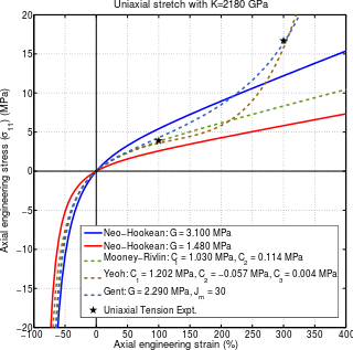
A hyperelastic or Green elastic material is a type of constitutive model for ideally elastic material for which the stress–strain relationship derives from a strain energy density function. The hyperelastic material is a special case of a Cauchy elastic material.

The derivation of the Navier–Stokes equations as well as its application and formulation for different families of fluids, is an important exercise in fluid dynamics with applications in mechanical engineering, physics, chemistry, heat transfer, and electrical engineering. A proof explaining the properties and bounds of the equations, such as Navier–Stokes existence and smoothness, is one of the important unsolved problems in mathematics.

The Cauchy momentum equation is a vector partial differential equation put forth by Cauchy that describes the non-relativistic momentum transport in any continuum.

<span class="mw-page-title-main">Deformation (physics)</span> Transformation of a body from a reference configuration to a current configuration

In physics and continuum mechanics, deformation is the change in the shape or size of an object. It has dimension of length with SI unit of metre (m). It is quantified as the residual displacement of particles in a non-rigid body, from an initial configuration to a final configuration, excluding the body's average translation and rotation. A configuration is a set containing the positions of all particles of the body.

In continuum mechanics, a compatible deformation tensor field in a body is that unique tensor field that is obtained when the body is subjected to a continuous, single-valued, displacement field. Compatibility is the study of the conditions under which such a displacement field can be guaranteed. Compatibility conditions are particular cases of integrability conditions and were first derived for linear elasticity by Barré de Saint-Venant in 1864 and proved rigorously by Beltrami in 1886.

In continuum mechanics, an Arruda–Boyce model is a hyperelastic constitutive model used to describe the mechanical behavior of rubber and other polymeric substances. This model is based on the statistical mechanics of a material with a cubic representative volume element containing eight chains along the diagonal directions. The material is assumed to be incompressible. The model is named after Ellen Arruda and Mary Cunningham Boyce, who published it in 1993.

The Gent hyperelastic material model is a phenomenological model of rubber elasticity that is based on the concept of limiting chain extensibility. In this model, the strain energy density function is designed such that it has a singularity when the first invariant of the left Cauchy-Green deformation tensor reaches a limiting value .

Curvilinear coordinates can be formulated in tensor calculus, with important applications in physics and engineering, particularly for describing transportation of physical quantities and deformation of matter in fluid mechanics and continuum mechanics.

<span class="mw-page-title-main">Objective stress rate</span>

In continuum mechanics, objective stress rates are time derivatives of stress that do not depend on the frame of reference. Many constitutive equations are designed in the form of a relation between a stress-rate and a strain-rate. The mechanical response of a material should not depend on the frame of reference. In other words, material constitutive equations should be frame-indifferent (objective). If the stress and strain measures are material quantities then objectivity is automatically satisfied. However, if the quantities are spatial, then the objectivity of the stress-rate is not guaranteed even if the strain-rate is objective.

References

  1. J. C. Simo and T. J. R. Hughes, 1998, Computational Inelasticity, Springer
  2. J. E. Marsden and T. J. R. Hughes, 2000, Mathematical Foundations of Elasticity, Dover.
  3. R. W. Ogden, 2000, Nonlinear Elastic Deformations, Dover.
  4. 1 2 Hjelmstad, Keith (2004). Fundamentals of Structural Mechanics. Springer Science & Business Media. p. 45. ISBN   9780387233307.