The Fresnel equations describe the reflection and transmission of light when incident on an interface between different optical media. They were deduced by French engineer and physicist Augustin-Jean Fresnel who was the first to understand that light is a transverse wave, when no one realized that the waves were electric and magnetic fields. For the first time, polarization could be understood quantitatively, as Fresnel's equations correctly predicted the differing behaviour of waves of the s and p polarizations incident upon a material interface.
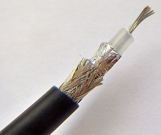
In electrical engineering, a transmission line is a specialized cable or other structure designed to conduct electromagnetic waves in a contained manner. The term applies when the conductors are long enough that the wave nature of the transmission must be taken into account. This applies especially to radio-frequency engineering because the short wavelengths mean that wave phenomena arise over very short distances. However, the theory of transmission lines was historically developed to explain phenomena on very long telegraph lines, especially submarine telegraph cables.
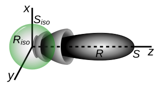
In electromagnetics, an antenna's gain is a key performance parameter which combines the antenna's directivity and radiation efficiency. The term power gain has been deprecated by IEEE. In a transmitting antenna, the gain describes how well the antenna converts input power into radio waves headed in a specified direction. In a receiving antenna, the gain describes how well the antenna converts radio waves arriving from a specified direction into electrical power. When no direction is specified, gain is understood to refer to the peak value of the gain, the gain in the direction of the antenna's main lobe. A plot of the gain as a function of direction is called the antenna pattern or radiation pattern. It is not to be confused with directivity, which does not take an antenna's radiation efficiency into account.
In mechanics and geometry, the 3D rotation group, often denoted SO(3), is the group of all rotations about the origin of three-dimensional Euclidean space under the operation of composition.

In physics and mathematics, the Lorentz group is the group of all Lorentz transformations of Minkowski spacetime, the classical and quantum setting for all (non-gravitational) physical phenomena. The Lorentz group is named for the Dutch physicist Hendrik Lorentz.

In electrical engineering, impedance matching is the practice of designing or adjusting the input impedance or output impedance of an electrical device for a desired value. Often, the desired value is selected to maximize power transfer or minimize signal reflection. For example, impedance matching typically is used to improve power transfer from a radio transmitter via the interconnecting transmission line to the antenna. Signals on a transmission line will be transmitted without reflections if the transmission line is terminated with a matching impedance.
In geodesy, conversion among different geographic coordinate systems is made necessary by the different geographic coordinate systems in use across the world and over time. Coordinate conversion is composed of a number of different types of conversion: format change of geographic coordinates, conversion of coordinate systems, or transformation to different geodetic datums. Geographic coordinate conversion has applications in cartography, surveying, navigation and geographic information systems.
Sound pressure or acoustic pressure is the local pressure deviation from the ambient atmospheric pressure, caused by a sound wave. In air, sound pressure can be measured using a microphone, and in water with a hydrophone. The SI unit of sound pressure is the pascal (Pa).
Particle velocity is the velocity of a particle in a medium as it transmits a wave. The SI unit of particle velocity is the metre per second (m/s). In many cases this is a longitudinal wave of pressure as with sound, but it can also be a transverse wave as with the vibration of a taut string.

In physics, the Rabi cycle is the cyclic behaviour of a two-level quantum system in the presence of an oscillatory driving field. A great variety of physical processes belonging to the areas of quantum computing, condensed matter, atomic and molecular physics, and nuclear and particle physics can be conveniently studied in terms of two-level quantum mechanical systems, and exhibit Rabi flopping when coupled to an optical driving field. The effect is important in quantum optics, magnetic resonance and quantum computing, and is named after Isidor Isaac Rabi.
In telecommunications, particularly in radio frequency engineering, signal strength refers to the transmitter power output as received by a reference antenna at a distance from the transmitting antenna. High-powered transmissions, such as those used in broadcasting, are expressed in dB-millivolts per metre (dBmV/m). For very low-power systems, such as mobile phones, signal strength is usually expressed in dB-microvolts per metre (dBμV/m) or in decibels above a reference level of one milliwatt (dBm). In broadcasting terminology, 1 mV/m is 1000 μV/m or 60 dBμ.
In linear algebra, linear transformations can be represented by matrices. If is a linear transformation mapping to and is a column vector with entries, then
In linear algebra, a rotation matrix is a transformation matrix that is used to perform a rotation in Euclidean space. For example, using the convention below, the matrix
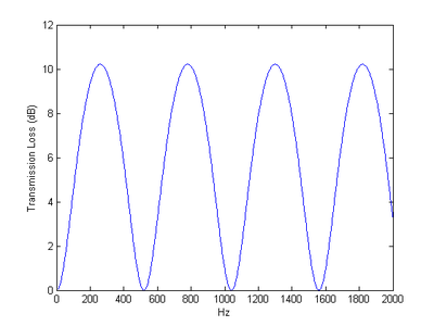
A sound attenuator, or duct silencer, sound trap, or muffler, is a noise control acoustical treatment of Heating Ventilating and Air-Conditioning (HVAC) ductwork designed to reduce transmission of noise through the ductwork, either from equipment into occupied spaces in a building, or between occupied spaces.

A transversely isotropic material is one with physical properties that are symmetric about an axis that is normal to a plane of isotropy. This transverse plane has infinite planes of symmetry and thus, within this plane, the material properties are the same in all directions. Hence, such materials are also known as "polar anisotropic" materials. In geophysics, vertically transverse isotropy (VTI) is also known as radial anisotropy.
Acoustic waves are a type of energy propagation through a medium by means of adiabatic loading and unloading. Important quantities for describing acoustic waves are acoustic pressure, particle velocity, particle displacement and acoustic intensity. Acoustic waves travel with a characteristic acoustic velocity that depends on the medium they're passing through. Some examples of acoustic waves are audible sound from a speaker, seismic waves, or ultrasound used for medical imaging.
Photon polarization is the quantum mechanical description of the classical polarized sinusoidal plane electromagnetic wave. An individual photon can be described as having right or left circular polarization, or a superposition of the two. Equivalently, a photon can be described as having horizontal or vertical linear polarization, or a superposition of the two.
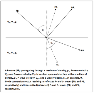
In geophysics and reflection seismology, the Zoeppritz equations are a set of equations that describe the partitioning of seismic wave energy at an interface, due to mode conversion. They are named after their author, the German geophysicist Karl Bernhard Zoeppritz, who died before they were published in 1919.

In mathematics, the axis–angle representation parameterizes a rotation in a three-dimensional Euclidean space by two quantities: a unit vector e indicating the direction (geometry) of an axis of rotation, and an angle of rotation θ describing the magnitude and sense of the rotation about the axis. Only two numbers, not three, are needed to define the direction of a unit vector e rooted at the origin because the magnitude of e is constrained. For example, the elevation and azimuth angles of e suffice to locate it in any particular Cartesian coordinate frame.
Transmission loss (TL) in general describes the accumulated decrease in intensity of a waveform energy as a wave propagates outwards from a source, or as it propagates through a certain area or through a certain type of structure.