Unit-weighted regression

Last updated March 06, 2024

In statistics, unit-weighted regression is a simplified and robust version (Wainer & Thissen, 1976) of multiple regression analysis where only the intercept term is estimated. That is, it fits a model

In the social sciences, unit-weighted regression is sometimes used for binary classification, i.e. to predict a yes-no answer where ${\hat {y}}<0$ indicates "no", ${\hat {y}}\geq 0$ "yes". It is easier to interpret than multiple linear regression (known as linear discriminant analysis in the classification case).

Unit weights

Unit-weighted regression is a method of robust regression that proceeds in three steps. First, predictors for the outcome of interest are selected; ideally, there should be good empirical or theoretical reasons for the selection. Second, the predictors are converted to a standard form. Finally, the predictors are added together, and this sum is called the variate, which is used as the predictor of the outcome.

Burgess method

The Burgess method was first presented by the sociologist Ernest W. Burgess in a 1928 study to determine success or failure of inmates placed on parole. First, he selected 21 variables believed to be associated with parole success. Next, he converted each predictor to the standard form of zero or one (Burgess, 1928). When predictors had two values, the value associated with the target outcome was coded as one. Burgess selected success on parole as the target outcome, so a predictor such as a history of theft was coded as "yes" = 0 and "no" = 1. These coded values were then added to create a predictor score, so that higher scores predicted a better chance of success. The scores could possibly range from zero (no predictors of success) to 21 (all 21 predictors scored as predicting success).

For predictors with more than two values, the Burgess method selects a cutoff score based on subjective judgment. As an example, a study using the Burgess method (Gottfredson & Snyder, 2005) selected as one predictor the number of complaints for delinquent behavior. With failure on parole as the target outcome, the number of complaints was coded as follows: "zero to two complaints" = 0, and "three or more complaints" = 1 (Gottfredson & Snyder, 2005. p. 18).

Kerby method

The Kerby method is similar to the Burgess method, but differs in two ways. First, while the Burgess method uses subjective judgment to select a cutoff score for a multi-valued predictor with a binary outcome, the Kerby method uses classification and regression tree (CART) analysis. In this way, the selection of the cutoff score is based not on subjective judgment, but on a statistical criterion, such as the point where the chi-square value is a maximum.

The second difference is that while the Burgess method is applied to a binary outcome, the Kerby method can apply to a multi-valued outcome, because CART analysis can identify cutoff scores in such cases, using a criterion such as the point where the t-value is a maximum. Because CART analysis is not only binary, but also recursive, the result can be that a predictor variable will be divided again, yielding two cutoff scores. The standard form for each predictor is that a score of one is added when CART analysis creates a partition.

One study (Kerby, 2003) selected as predictors the five traits of the Big five personality traits, predicting a multi-valued measure of suicidal ideation. Next, the personality scores were converted into standard form with CART analysis. When the CART analysis yielded one partition, the result was like the Burgess method in that the predictor was coded as either zero or one. But for the measure of neuroticism, the result was two cutoff scores. Because higher neuroticism scores correlated with more suicidal thinking, the two cutoff scores led to the following coding: "low Neuroticism" = 0, "moderate Neuroticism" = 1, "high Neuroticism" = 2 (Kerby, 2003).

z-score method

Another method can be applied when the predictors are measured on a continuous scale. In such a case, each predictor can be converted into a standard score, or z-score, so that all the predictors have a mean of zero and a standard deviation of one. With this method of unit-weighted regression, the variate is a sum of the z-scores (e.g., Dawes, 1979; Bobko, Roth, & Buster, 2007).

Literature review

The first empirical study using unit-weighted regression is widely considered to be a 1928 study by sociologist Ernest W. Burgess. He used 21 variables to predict parole success or failure, and the results suggest that unit weights are a useful tool in making decisions about which inmates to parole. Of those inmates with the best scores, 98% did in fact succeed on parole; and of those with the worst scores, only 24% did in fact succeed (Burgess, 1928).

The mathematical issues involved in unit-weighted regression were first discussed in 1938 by Samuel Stanley Wilks, a leading statistician who had a special interest in multivariate analysis. Wilks described how unit weights could be used in practical settings, when data were not available to estimate beta weights. For example, a small college may want to select good students for admission. But the school may have no money to gather data and conduct a standard multiple regression analysis. In this case, the school could use several predictors—high school grades, SAT scores, teacher ratings. Wilks (1938) showed mathematically why unit weights should work well in practice.

Frank Schmidt (1971) conducted a simulation study of unit weights. His results showed that Wilks was indeed correct and that unit weights tend to perform well in simulations of practical studies.

Robyn Dawes (1979) discussed the use of unit weights in applied studies, referring to the robust beauty of unit weighted models. Jacob Cohen also discussed the value of unit weights and noted their practical utility. Indeed, he wrote, "As a practical matter, most of the time, we are better off using unit weights" (Cohen, 1990, p. 1306).

Dave Kerby (2003) showed that unit weights compare well with standard regression, doing so with a cross validation study—that is, he derived beta weights in one sample and applied them to a second sample. The outcome of interest was suicidal thinking, and the predictor variables were broad personality traits. In the cross validation sample, the correlation between personality and suicidal thinking was slightly stronger with unit-weighted regression (r = .48) than with standard multiple regression (r = .47).

Gottfredson and Snyder (2005) compared the Burgess method of unit-weighted regression to other methods, with a construction sample of N = 1,924 and a cross-validation sample of N = 7,552. Using the Pearson point-biserial, the effect size in the cross validation sample for the unit-weights model was r = .392, which was somewhat larger than for logistic regression (r = .368) and predictive attribute analysis (r = .387), and less than multiple regression only in the third decimal place (r = .397).

In a review of the literature on unit weights, Bobko, Roth, and Buster (2007) noted that "unit weights and regression weights perform similarly in terms of the magnitude of cross-validated multiple correlation, and empirical studies have confirmed this result across several decades" (p. 693).

Andreas Graefe applied an equal weighting approach to nine established multiple regression models for forecasting U.S. presidential elections. Across the ten elections from 1976 to 2012, equally weighted predictors reduced the forecast error of the original regression models on average by four percent. An equal-weights model that includes all variables provided calibrated forecasts that reduced the error of the most accurate regression model by 29% percent.^[1]

Example

An example may clarify how unit weights can be useful in practice.

Brenna Bry and colleagues (1982) addressed the question of what causes drug use in adolescents. Previous research had made use of multiple regression; with this method, it is natural to look for the best predictor, the one with the highest beta weight. Bry and colleagues noted that one previous study had found that early use of alcohol was the best predictor. Another study had found that alienation from parents was the best predictor. Still another study had found that low grades in school were the best predictor. The failure to replicate was clearly a problem, a problem that could be caused by bouncing betas.

Bry and colleagues suggested a different approach: instead of looking for the best predictor, they looked at the number of predictors. In other words, they gave a unit weight to each predictor. Their study had six predictors: 1) low grades in school, 2) lack of affiliation with religion, 3) early age of alcohol use, 4) psychological distress, 5) low self-esteem, and 6) alienation from parents. To convert the predictors to standard form, each risk factor was scored as absent (scored as zero) or present (scored as one). For example, the coding for low grades in school were as follows: "C or higher" = 0, "D or F" = 1. The results showed that the number of risk factors was a good predictor of drug use: adolescents with more risk factors were more likely to use drugs.

The model used by Bry and colleagues was that drug users do not differ in any special way from non-drug users. Rather, they differ in the number of problems they must face. "The number of factors an individual must cope with is more important than exactly what those factors are" (p. 277). Given this model, unit-weighted regression is an appropriate method of analysis.

Beta weights

In standard multiple regression, each predictor is multiplied by a number that is called the beta weight, regression weight or weighted regression coefficients (denoted β_W or BW).^[2] The prediction is obtained by adding these products along with a constant. When the weights are chosen to give the best prediction by some criterion, the model referred to as a proper linear model. Therefore, multiple regression is a proper linear model. By contrast, unit-weighted regression is called an improper linear model.

Model specification

Standard multiple regression hinges on the assumption that all relevant predictors of the outcome are included in the regression model. This assumption is called model specification. A model is said to be specified when all relevant predictors are included in the model, and all irrelevant predictors are excluded from the model. In practical settings, it is rare for a study to be able to determine all relevant predictors a priori. In this case, models are not specified and the estimates for the beta weights suffer from omitted variable bias. That is, the beta weights may change from one sample to the next, a situation sometimes called the problem of the bouncing betas. It is this problem with bouncing betas that makes unit-weighted regression a useful method.

Related Research Articles

The method of least squares is a parameter estimation method in regression analysis based on minimizing the sum of the squares of the residuals made in the results of each individual equation.

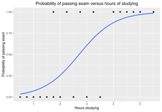
In statistics, the logistic model is a statistical model that models the log-odds of an event as a linear combination of one or more independent variables. In regression analysis, logistic regression is estimating the parameters of a logistic model. Formally, in binary logistic regression there is a single binary dependent variable, coded by an indicator variable, where the two values are labeled "0" and "1", while the independent variables can each be a binary variable or a continuous variable. The corresponding probability of the value labeled "1" can vary between 0 and 1, hence the labeling; the function that converts log-odds to probability is the logistic function, hence the name. The unit of measurement for the log-odds scale is called a logit, from logistic unit, hence the alternative names. See § Background and § Definition for formal mathematics, and § Example for a worked example.

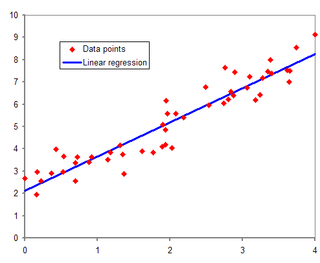
In statistical modeling, regression analysis is a set of statistical processes for estimating the relationships between a dependent variable and one or more independent variables. The most common form of regression analysis is linear regression, in which one finds the line that most closely fits the data according to a specific mathematical criterion. For example, the method of ordinary least squares computes the unique line that minimizes the sum of squared differences between the true data and that line. For specific mathematical reasons, this allows the researcher to estimate the conditional expectation of the dependent variable when the independent variables take on a given set of values. Less common forms of regression use slightly different procedures to estimate alternative location parameters or estimate the conditional expectation across a broader collection of non-linear models.

The general linear model or general multivariate regression model is a compact way of simultaneously writing several multiple linear regression models. In that sense it is not a separate statistical linear model. The various multiple linear regression models may be compactly written as

In statistics, nonlinear regression is a form of regression analysis in which observational data are modeled by a function which is a nonlinear combination of the model parameters and depends on one or more independent variables. The data are fitted by a method of successive approximations.

In statistics, the coefficient of determination, denoted R² or r² and pronounced "R squared", is the proportion of the variation in the dependent variable that is predictable from the independent variable(s).

In statistics, classification is the problem of identifying which of a set of categories (sub-populations) an observation belongs to. Examples are assigning a given email to the "spam" or "non-spam" class, and assigning a diagnosis to a given patient based on observed characteristics of the patient.

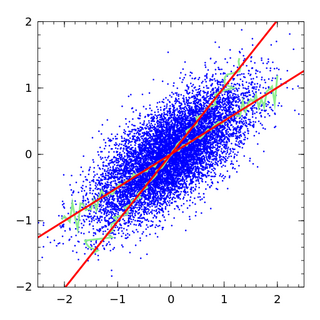
Regression dilution, also known as regression attenuation, is the biasing of the linear regression slope towards zero, caused by errors in the independent variable.

In statistics, Poisson regression is a generalized linear model form of regression analysis used to model count data and contingency tables. Poisson regression assumes the response variable Y has a Poisson distribution, and assumes the logarithm of its expected value can be modeled by a linear combination of unknown parameters. A Poisson regression model is sometimes known as a log-linear model, especially when used to model contingency tables.

In robust statistics, robust regression seeks to overcome some limitations of traditional regression analysis. A regression analysis models the relationship between one or more independent variables and a dependent variable. Standard types of regression, such as ordinary least squares, have favourable properties if their underlying assumptions are true, but can give misleading results otherwise. Robust regression methods are designed to limit the effect that violations of assumptions by the underlying data-generating process have on regression estimates.

Ernest Watson Burgess was a Canadian-American urban sociologist born in Tilbury, Ontario. He was educated at Kingfisher College in Oklahoma and continued graduate studies in sociology at the University of Chicago. In 1916, he returned to the University of Chicago, as a faculty member. Burgess was hired as an urban sociologist at the University of Chicago. Burgess also served as the 24th President of the American Sociological Association (ASA).

In statistics, multinomial logistic regression is a classification method that generalizes logistic regression to multiclass problems, i.e. with more than two possible discrete outcomes. That is, it is a model that is used to predict the probabilities of the different possible outcomes of a categorically distributed dependent variable, given a set of independent variables.

A mixed model, mixed-effects model or mixed error-component model is a statistical model containing both fixed effects and random effects. These models are useful in a wide variety of disciplines in the physical, biological and social sciences. They are particularly useful in settings where repeated measurements are made on the same statistical units, or where measurements are made on clusters of related statistical units. Mixed models are often preferred over traditional analysis of variance regression models because of their flexibility in dealing with missing values and uneven spacing of repeated measurements. The Mixed model analysis allows measurements to be explicitly modeled in a wider variety of correlation and variance-covariance structures.

In statistics, standardized (regression) coefficients, also called beta coefficients or beta weights, are the estimates resulting from a regression analysis where the underlying data have been standardized so that the variances of dependent and independent variables are equal to 1. Therefore, standardized coefficients are unitless and refer to how many standard deviations a dependent variable will change, per standard deviation increase in the predictor variable.

Demand forecasting refers to the process of predicting the quantity of goods and services that will be demanded by consumers at a future point in time. More specifically, the methods of demand forecasting entail using predictive analytics to estimate customer demand in consideration of key economic conditions. This is an important tool in optimizing business profitability through efficient supply chain management. Demand forecasting methods are divided into two major categories, qualitative and quantitative methods. Qualitative methods are based on expert opinion and information gathered from the field. This method is mostly used in situations when there is minimal data available for analysis such as when a business or product has recently been introduced to the market. Quantitative methods, however, use available data, and analytical tools in order to produce predictions. Demand forecasting may be used in resource allocation, inventory management, assessing future capacity requirements, or making decisions on whether to enter a new market.

Linear least squares (LLS) is the least squares approximation of linear functions to data. It is a set of formulations for solving statistical problems involved in linear regression, including variants for ordinary (unweighted), weighted, and generalized (correlated) residuals. Numerical methods for linear least squares include inverting the matrix of the normal equations and orthogonal decomposition methods.

In statistics and in machine learning, a linear predictor function is a linear function of a set of coefficients and explanatory variables, whose value is used to predict the outcome of a dependent variable. This sort of function usually comes in linear regression, where the coefficients are called regression coefficients. However, they also occur in various types of linear classifiers, as well as in various other models, such as principal component analysis and factor analysis. In many of these models, the coefficients are referred to as "weights".

In statistics, linear regression is a statistical model which estimates the linear relationship between a scalar response and one or more explanatory variables. The case of one explanatory variable is called simple linear regression; for more than one, the process is called multiple linear regression. This term is distinct from multivariate linear regression, where multiple correlated dependent variables are predicted, rather than a single scalar variable. If the explanatory variables are measured with error then errors-in-variables models are required, also known as measurement error models.

In statistics, specifically regression analysis, a binary regression estimates a relationship between one or more explanatory variables and a single output binary variable. Generally the probability of the two alternatives is modeled, instead of simply outputting a single value, as in linear regression.

Non-homogeneous Gaussian regression (NGR) is a type of statistical regression analysis used in the atmospheric sciences as a way to convert ensemble forecasts into probabilistic forecasts. Relative to simple linear regression, NGR uses the ensemble spread as an additional predictor, which is used to improve the prediction of uncertainty and allows the predicted uncertainty to vary from case to case. The prediction of uncertainty in NGR is derived from both past forecast errors statistics and the ensemble spread. NGR was originally developed for site-specific medium range temperature forecasting, but has since also been applied to site-specific medium-range wind forecasting and to seasonal forecasts, and has been adapted for precipitation forecasting. The introduction of NGR was the first demonstration that probabilistic forecasts that take account of the varying ensemble spread could achieve better skill scores than forecasts based on standard Model output statistics approaches applied to the ensemble mean.

References

↑ Graefe, Andreas (2015). "Improving forecasts using equally weighted predictors" (PDF). Journal of Business Research. Elsevier. 68 (8): 1792–1799. doi:10.1016/j.jbusres.2015.03.038.
↑ Ziglari, Leily (2017). "Interpreting Multiple Regression Results: β Weights and Structure Coefficients" (PDF). General Linear Model Journal. GLMJ. 43 (1): 13–22. doi:10.31523/glmj.043002.002.

Bobko, P., Roth, P. L., & Buster, M. A. (2007). "The usefulness of unit weights in creating composite scores: A literature review, application to content validity, and meta-analysis". Organizational Research Methods, volume 10, pages 689-709. doi : 10.1177/1094428106294734
Bry, B. H.; McKeon, P.; Pandina, R. J. (1982). "Extent of drug use as a function of number of risk factors". Journal of Abnormal Psychology. 91 (4): 273–279. doi:10.1037/0021-843X.91.4.273. PMID 7130523.
Burgess, E. W. (1928). "Factors determining success or failure on parole". In A. A. Bruce (Ed.), The Workings of the Indeterminate Sentence Law and Parole in Illinois (pp. 205–249). Springfield, Illinois: Illinois State Parole Board. Google books
Cohen, Jacob. (1990). "Things I have learned (so far)". American Psychologist, volume 45, pages 1304-1312. doi : 10.1037/0003-066X.45.12.1304
Dawes, Robyn M. (1979). "The robust beauty of improper linear models in decision making". American Psychologist, volume 34, pages 571-582. doi : 10.1037/0003-066X.34.7.571. archived pdf
Gottfredson, D. M., & Snyder, H. N. (July 2005). The mathematics of risk classification: Changing data into valid instruments for juvenile courts. Pittsburgh, Penn.: National Center for Juvenile Justice. NCJ 209158. Eric.ed.gov pdf
Kerby, Dave S. (2003). "CART analysis with unit-weighted regression to predict suicidal ideation from Big Five traits". Personality and Individual Differences, volume 35, pages 249-261. doi : 10.1016/S0191-8869(02)00174-5
Schmidt, Frank L. (1971). "The relative efficiency of regression and simple unit predictor weights in applied differential psychology". Educational and Psychological Measurement, volume 31, pages 699-714. doi : 10.1177/001316447103100310
Wainer, H., & Thissen, D. (1976). Three steps toward robust regression. Psychometrika, volume 41(1), pages 9–34. doi : 10.1007/BF02291695
Wilks, S. S. (1938). "Weighting systems for linear functions of correlated variables when there is no dependent variable". Psychometrika. 3: 23–40. doi:10.1007/BF02287917.

External links

Chis Stucchio blog - Why a pro/con list is 75% as good as your fancy machine learning algorithm

This page is based on this Wikipedia article
Text is available under the CC BY-SA 4.0 license; additional terms may apply.
Images, videos and audio are available under their respective licenses.

[1] Graefe, Andreas (2015). "Improving forecasts using equally weighted predictors" (PDF). Journal of Business Research. Elsevier. 68 (8): 1792–1799. doi:10.1016/j.jbusres.2015.03.038.

[2] Ziglari, Leily (2017). "Interpreting Multiple Regression Results: β Weights and Structure Coefficients" (PDF). General Linear Model Journal. GLMJ. 43 (1): 13–22. doi:10.31523/glmj.043002.002.

[1]

[2]