Unpolarized light

Last updated August 01, 2023

Unpolarized light is light with a random, time-varying polarization. Natural light, like most other common sources of visible light, is produced independently by a large number of atoms or molecules whose emissions are uncorrelated. This term is somewhat inexact, since at any instant of time at one location there is a definite plane of polarization; however, it implies that the polarization changes so quickly in time that it will not be measured or relevant to the outcome of an experiment.

Unpolarized light can be produced from the incoherent combination of vertical and horizontal linearly polarized light, or right- and left-handed circularly polarized light.^[1] Conversely, the two constituent linearly polarized states of unpolarized light cannot form an interference pattern, even if rotated into alignment (Fresnel–Arago 3rd law).^[2]

A so-called depolarizer acts on a polarized beam to create one in which the polarization varies so rapidly across the beam that it may be ignored in the intended applications. Conversely, a polarizer acts on an unpolarized beam or arbitrarily polarized beam to create one which is polarized.

Unpolarized light can be described as a mixture of two independent oppositely polarized streams, each with half the intensity.^[3]^[4] Light is said to be partially polarized when there is more power in one of these streams than the other. At any particular wavelength, partially polarized light can be statistically described as the superposition of a completely unpolarized component and a completely polarized one.^[5]^{: 346–347}^[6]^: 330 One may then describe the light in terms of the degree of polarization and the parameters of the polarized component. That polarized component can be described in terms of a Jones vector or polarization ellipse. However, in order to also describe the degree of polarization, one normally employs Stokes parameters to specify a state of partial polarization.^[5]^{: 351, 374–375}

Motivation

The transmission of plane waves through a homogeneous medium are fully described in terms of Jones vectors and 2×2 Jones matrices. However, in practice there are cases in which all of the light cannot be viewed in such a simple manner due to spatial inhomogeneities or the presence of mutually incoherent waves. So-called depolarization, for instance, cannot be described using Jones matrices. For these cases it is usual instead to use a 4×4 matrix that acts upon the Stokes 4-vector. Such matrices were first used by Paul Soleillet in 1929, although they have come to be known as Mueller matrices. While every Jones matrix has a Mueller matrix, the reverse is not true. Mueller matrices are then used to describe the observed polarization effects of the scattering of waves from complex surfaces or ensembles of particles, as shall now be presented.^[5]^{: 377–379}

Coherency matrix

The Jones vector perfectly describes the state of polarization and phase of a single monochromatic wave, representing a pure state of polarization as described above. However any mixture of waves of different polarizations (or even of different frequencies) do not correspond to a Jones vector. In so-called partially polarized radiation the fields are stochastic, and the variations and correlations between components of the electric field can only be described statistically. One such representation is the coherency matrix :^[7]^{: 137–142}

{\begin{aligned}\mathbf {\Psi } &=\left\langle \mathbf {e} \mathbf {e} ^{\dagger }\right\rangle \\&=\left\langle {\begin{bmatrix}e_{1}e_{1}^{*}&e_{1}e_{2}^{*}\\e_{2}e_{1}^{*}&e_{2}e_{2}^{*}\end{bmatrix}}\right\rangle \\&=\left\langle {\begin{bmatrix}a_{1}^{2}&a_{1}a_{2}e^{i\left(\theta _{1}-\theta _{2}\right)}\\a_{1}a_{2}e^{-i\left(\theta _{1}-\theta _{2}\right)}&a_{2}^{2}\end{bmatrix}}\right\rangle \end{aligned}}

where angular brackets denote averaging over many wave cycles. Several variants of the coherency matrix have been proposed: the Wiener coherency matrix and the spectral coherency matrix of Richard Barakat measure the coherence of a spectral decomposition of the signal, while the Wolf coherency matrix averages over all time/frequencies.

The coherency matrix contains all second order statistical information about the polarization. This matrix can be decomposed into the sum of two idempotent matrices, corresponding to the eigenvectors of the coherency matrix, each representing a polarization state that is orthogonal to the other. An alternative decomposition is into completely polarized (zero determinant) and unpolarized (scaled identity matrix) components. In either case, the operation of summing the components corresponds to the incoherent superposition of waves from the two components. The latter case gives rise to the concept of the "degree of polarization"; i.e., the fraction of the total intensity contributed by the completely polarized component.

Stokes parameters

The coherency matrix is not easy to visualize, and it is therefore common to describe incoherent or partially polarized radiation in terms of its total intensity (I), (fractional) degree of polarization (p), and the shape parameters of the polarization ellipse. An alternative and mathematically convenient description is given by the Stokes parameters, introduced by George Gabriel Stokes in 1852. The relationship of the Stokes parameters to intensity and polarization ellipse parameters is shown in the equations and figure below.

S_{0}=I\,

S_{1}=Ip\cos 2\psi \cos 2\chi \,

S_{2}=Ip\sin 2\psi \cos 2\chi \,

S_{3}=Ip\sin 2\chi \,

Here Ip, 2ψ and 2χ are the spherical coordinates of the polarization state in the three-dimensional space of the last three Stokes parameters. Note the factors of two before ψ and χ corresponding respectively to the facts that any polarization ellipse is indistinguishable from one rotated by 180°, or one with the semi-axis lengths swapped accompanied by a 90° rotation. The Stokes parameters are sometimes denoted I, Q, U and V.

The four Stokes parameters are enough to describe 2D polarization of a paraxial wave, but not the 3D polarization of a general non-paraxial wave or an evanescent field.^[8]^[9]

Poincaré sphere

Neglecting the first Stokes parameter S₀ (or I), the three other Stokes parameters can be plotted directly in three-dimensional Cartesian coordinates. For a given power in the polarized component given by

P={\sqrt {S_{1}^{2}+S_{2}^{2}+S_{3}^{2}}}

the set of all polarization states are then mapped to points on the surface of the so-called Poincaré sphere (but of radius P), as shown in the accompanying diagram.

Depiction of the polarization states on Poincare sphere Poincaresp.png — Depiction of the polarization states on Poincaré sphere

Often the total beam power is not of interest, in which case a normalized Stokes vector is used by dividing the Stokes vector by the total intensity S₀:

\mathbf {S'} ={\frac {1}{S_{0}}}{\begin{bmatrix}S_{0}\\S_{1}\\S_{2}\\S_{3}\end{bmatrix}}.

The normalized Stokes vector $\mathbf {S'}$ then has unity power ( $S'_{0}=1$ ) and the three significant Stokes parameters plotted in three dimensions will lie on the unity-radius Poincaré sphere for pure polarization states (where $P'_{0}=1$ ). Partially polarized states will lie inside the Poincaré sphere at a distance of $P'={\sqrt {S_{1}'^{2}+S_{2}'^{2}+S_{3}'^{2}}}$ from the origin. When the non-polarized component is not of interest, the Stokes vector can be further normalized to obtain

\mathbf {S''} ={\frac {1}{P'}}{\begin{bmatrix}1\\S'_{1}\\S'_{2}\\S'_{3}\end{bmatrix}}={\frac {1}{P}}{\begin{bmatrix}S_{0}\\S_{1}\\S_{2}\\S_{3}\end{bmatrix}}.

When plotted, that point will lie on the surface of the unity-radius Poincaré sphere and indicate the state of polarization of the polarized component.

Any two antipodal points on the Poincaré sphere refer to orthogonal polarization states. The overlap between any two polarization states is dependent solely on the distance between their locations along the sphere. This property, which can only be true when pure polarization states are mapped onto a sphere, is the motivation for the invention of the Poincaré sphere and the use of Stokes parameters, which are thus plotted on (or beneath) it.

Note that the IEEE defines RHCP and LHCP the opposite as those used by Physicists. The IEEE 1979 Antenna Standard will show RHCP on the South Pole of the Poincare Sphere. The IEEE defines RHCP using the right hand with thumb pointing in the direction of transmit, and the fingers showing the direction of rotation of the E field with time. The rationale for the opposite conventions used by Physicists and Engineers is that Astronomical Observations are always done with the incoming wave traveling toward the observer, where as for most engineers, they are assumed to be standing behind the transmitter watching the wave traveling away from them. This article is not using the IEEE 1979 Antenna Standard and is not using the +t convention typically used in IEEE work.

Related Research Articles

The Fresnel equations describe the reflection and transmission of light when incident on an interface between different optical media. They were deduced by Augustin-Jean Fresnel who was the first to understand that light is a transverse wave, even though no one realized that the "vibrations" of the wave were electric and magnetic fields. For the first time, polarization could be understood quantitatively, as Fresnel's equations correctly predicted the differing behaviour of waves of the s and p polarizations incident upon a material interface.

In optics, polarized light can be described using the Jones calculus, discovered by R. C. Jones in 1941. Polarized light is represented by a Jones vector, and linear optical elements are represented by Jones matrices. When light crosses an optical element the resulting polarization of the emerging light is found by taking the product of the Jones matrix of the optical element and the Jones vector of the incident light. Note that Jones calculus is only applicable to light that is already fully polarized. Light which is randomly polarized, partially polarized, or incoherent must be treated using Mueller calculus.

In mathematical physics and mathematics, the Pauli matrices are a set of three $2 \times 2$ complex matrices which are Hermitian, involutory and unitary. Usually indicated by the Greek letter sigma, they are occasionally denoted by tau when used in connection with isospin symmetries.

<span class="mw-page-title-main">Circular polarization</span> Polarization state

In electrodynamics, circular polarization of an electromagnetic wave is a polarization state in which, at each point, the electromagnetic field of the wave has a constant magnitude and is rotating at a constant rate in a plane perpendicular to the direction of the wave.

In electrodynamics, elliptical polarization is the polarization of electromagnetic radiation such that the tip of the electric field vector describes an ellipse in any fixed plane intersecting, and normal to, the direction of propagation. An elliptically polarized wave may be resolved into two linearly polarized waves in phase quadrature, with their polarization planes at right angles to each other. Since the electric field can rotate clockwise or counterclockwise as it propagates, elliptically polarized waves exhibit chirality.

<span class="mw-page-title-main">Polarization (physics)</span> Property of waves that can oscillate with more than one orientation

Polarization is a property of transverse waves which specifies the geometrical orientation of the oscillations. In a transverse wave, the direction of the oscillation is perpendicular to the direction of motion of the wave. A simple example of a polarized transverse wave is vibrations traveling along a taut string (see image); for example, in a musical instrument like a guitar string. Depending on how the string is plucked, the vibrations can be in a vertical direction, horizontal direction, or at any angle perpendicular to the string. In contrast, in longitudinal waves, such as sound waves in a liquid or gas, the displacement of the particles in the oscillation is always in the direction of propagation, so these waves do not exhibit polarization. Transverse waves that exhibit polarization include electromagnetic waves such as light and radio waves, gravitational waves, and transverse sound waves in solids.

<span class="mw-page-title-main">Waveplate</span> Optical polarization device

A waveplate or retarder is an optical device that alters the polarization state of a light wave travelling through it. Two common types of waveplates are the half-wave plate, which shifts the polarization direction of linearly polarized light, and the quarter-wave plate, which converts linearly polarized light into circularly polarized light and vice versa. A quarter-wave plate can be used to produce elliptical polarization as well.

In physics and mathematics, the Lorentz group is the group of all Lorentz transformations of Minkowski spacetime, the classical and quantum setting for all (non-gravitational) physical phenomena. The Lorentz group is named for the Dutch physicist Hendrik Lorentz.

In quantum field theory, the Dirac spinor is the spinor that describes all known fundamental particles that are fermions, with the possible exception of neutrinos. It appears in the plane-wave solution to the Dirac equation, and is a certain combination of two Weyl spinors, specifically, a bispinor that transforms "spinorially" under the action of the Lorentz group.

In linear algebra, linear transformations can be represented by matrices. If $is a linear transformation mapping to and is a column vector with entries, then$

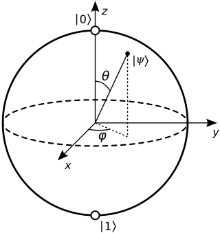
In quantum mechanics and computing, the Bloch sphere is a geometrical representation of the pure state space of a two-level quantum mechanical system (qubit), named after the physicist Felix Bloch.

In linear algebra, a rotation matrix is a transformation matrix that is used to perform a rotation in Euclidean space. For example, using the convention below, the matrix

In mathematics, an ordered basis of a vector space of finite dimension $n$ allows representing uniquely any element of the vector space by a coordinate vector, which is a sequence of $n$ scalars called coordinates. If two different bases are considered, the coordinate vector that represents a vector $v$ on one basis is, in general, different from the coordinate vector that represents $v$ on the other basis. A change of basis consists of converting every assertion expressed in terms of coordinates relative to one basis into an assertion expressed in terms of coordinates relative to the other basis.

The Stokes parameters are a set of values that describe the polarization state of electromagnetic radiation. They were defined by George Gabriel Stokes in 1852, as a mathematically convenient alternative to the more common description of incoherent or partially polarized radiation in terms of its total intensity (I), (fractional) degree of polarization (p), and the shape parameters of the polarization ellipse. The effect of an optical system on the polarization of light can be determined by constructing the Stokes vector for the input light and applying Mueller calculus, to obtain the Stokes vector of the light leaving the system. The original Stokes paper was discovered independently by Francis Perrin in 1942 and by Subrahamanyan Chandrasekhar in 1947, who named it as the Stokes parameters.

In linear algebra, an eigenvector or characteristic vector of a linear transformation is a nonzero vector that changes at most by a constant factor when that linear transformation is applied to it. The corresponding eigenvalue, often represented by $, is the multiplying factor.$

Mueller calculus is a matrix method for manipulating Stokes vectors, which represent the polarization of light. It was developed in 1943 by Hans Mueller. In this technique, the effect of a particular optical element is represented by a Mueller matrix—a 4×4 matrix that is an overlapping generalization of the Jones matrix.

Sinusoidal plane-wave solutions are particular solutions to the electromagnetic wave equation.

In geometry, various formalisms exist to express a rotation in three dimensions as a mathematical transformation. In physics, this concept is applied to classical mechanics where rotational kinematics is the science of quantitative description of a purely rotational motion. The orientation of an object at a given instant is described with the same tools, as it is defined as an imaginary rotation from a reference placement in space, rather than an actually observed rotation from a previous placement in space.

In fluid dynamics, the Oseen equations describe the flow of a viscous and incompressible fluid at small Reynolds numbers, as formulated by Carl Wilhelm Oseen in 1910. Oseen flow is an improved description of these flows, as compared to Stokes flow, with the (partial) inclusion of convective acceleration.

Symmetries in quantum mechanics describe features of spacetime and particles which are unchanged under some transformation, in the context of quantum mechanics, relativistic quantum mechanics and quantum field theory, and with applications in the mathematical formulation of the standard model and condensed matter physics. In general, symmetry in physics, invariance, and conservation laws, are fundamentally important constraints for formulating physical theories and models. In practice, they are powerful methods for solving problems and predicting what can happen. While conservation laws do not always give the answer to the problem directly, they form the correct constraints and the first steps to solving a multitude of problems.

References

↑ Chipman, R.A.; Lam, W.S.T.; Young, G. (2018). Polarized Light and Optical Systems. Optical Sciences and Applications of Light. CRC Press. ISBN 978-1-4987-0057-3 . Retrieved 2023-01-20.
↑ Sharma, K.K. (2006). Optics: Principles and Applications. Elsevier Science. p. 145. ISBN 978-0-08-046391-9 . Retrieved 2023-01-20.
↑ Prakash, Hari; Chandra, Naresh (1971). "Density Operator of Unpolarized Radiation". Physical Review A. 4 (2): 796–799. Bibcode:1971PhRvA...4..796P. doi:10.1103/PhysRevA.4.796.
↑ Chandrasekhar, Subrahmanyan (2013). Radiative transfer. Courier. p. 30.
1 2 3 Hecht, Eugene (2002). Optics (4th ed.). United States of America: Addison Wesley. ISBN 0-8053-8566-5.
↑ Bekefi, George; Barrett, Alan (1977). Electromagnetic Vibrations, Waves, and Radiation . USA: MIT Press. ISBN 0-262-52047-8.
↑ Edward L. O'Neill (January 2004). Introduction to Statistical Optics. Courier Dover Publications. ISBN 978-0-486-43578-7.
↑ Eismann, J. S.; Nicholls, L. H.; Roth, D. J.; Alonso, M. A.; Banzer, P.; Rodríguez-Fortuño, F. J.; Zayats, A. V.; Nori, F.; Bliokh, K. Y. (2021). "Transverse spinning of unpolarized light". Nature Photonics. 15 (2): 156–161. arXiv: 2004.02970 . Bibcode:2021NaPho..15..156E. doi:10.1038/s41566-020-00733-3. ISSN 1749-4885. S2CID 215238513.
↑ Sugic, Danica; Dennis, Mark R.; Nori, Franco; Bliokh, Konstantin Y. (2020-12-23). "Knotted polarizations and spin in three-dimensional polychromatic waves". Physical Review Research. 2 (4): 042045. arXiv: 2007.13307 . Bibcode:2020PhRvR...2d2045S. doi: 10.1103/PhysRevResearch.2.042045 . ISSN 2643-1564.

This page is based on this Wikipedia article
Text is available under the CC BY-SA 4.0 license; additional terms may apply.
Images, videos and audio are available under their respective licenses.

[Chipman_Lam_Young_2018_p.-1] Chipman, R.A.; Lam, W.S.T.; Young, G. (2018). Polarized Light and Optical Systems. Optical Sciences and Applications of Light. CRC Press. ISBN 978-1-4987-0057-3 . Retrieved 2023-01-20.

[Sharma_2006_p._145-2] Sharma, K.K. (2006). Optics: Principles and Applications. Elsevier Science. p. 145. ISBN 978-0-08-046391-9 . Retrieved 2023-01-20.

[3] Prakash, Hari; Chandra, Naresh (1971). "Density Operator of Unpolarized Radiation". Physical Review A. 4 (2): 796–799. Bibcode:1971PhRvA...4..796P. doi:10.1103/PhysRevA.4.796.

[4] Chandrasekhar, Subrahmanyan (2013). Radiative transfer. Courier. p. 30.

[Hecht2002-5] 1 2 3 Hecht, Eugene (2002). Optics (4th ed.). United States of America: Addison Wesley. ISBN 0-8053-8566-5.

[Bekefi-6] Bekefi, George; Barrett, Alan (1977). Electromagnetic Vibrations, Waves, and Radiation . USA: MIT Press. ISBN 0-262-52047-8.

[O'Neill2004-7] Edward L. O'Neill (January 2004). Introduction to Statistical Optics. Courier Dover Publications. ISBN 978-0-486-43578-7.

[8] Eismann, J. S.; Nicholls, L. H.; Roth, D. J.; Alonso, M. A.; Banzer, P.; Rodríguez-Fortuño, F. J.; Zayats, A. V.; Nori, F.; Bliokh, K. Y. (2021). "Transverse spinning of unpolarized light". Nature Photonics. 15 (2): 156–161. arXiv: 2004.02970 . Bibcode:2021NaPho..15..156E. doi:10.1038/s41566-020-00733-3. ISSN 1749-4885. S2CID 215238513.

[9] Sugic, Danica; Dennis, Mark R.; Nori, Franco; Bliokh, Konstantin Y. (2020-12-23). "Knotted polarizations and spin in three-dimensional polychromatic waves". Physical Review Research. 2 (4): 042045. arXiv: 2007.13307 . Bibcode:2020PhRvR...2d2045S. doi: 10.1103/PhysRevResearch.2.042045 . ISSN 2643-1564.

[1]

[2]

[3]

[4]

[5]

[6]

[7]

[8]

[9]