
In mathematics, Stirling's approximation is an asymptotic approximation for factorials. It is a good approximation, leading to accurate results even for small values of . It is named after James Stirling, though a related but less precise result was first stated by Abraham de Moivre.

In statistical mechanics and information theory, the Fokker–Planck equation is a partial differential equation that describes the time evolution of the probability density function of the velocity of a particle under the influence of drag forces and random forces, as in Brownian motion. The equation can be generalized to other observables as well. The Fokker-Planck equation has multiple applications in information theory, graph theory, data science, finance, economics etc.
Fractional calculus is a branch of mathematical analysis that studies the several different possibilities of defining real number powers or complex number powers of the differentiation operator

In relativity, proper time along a timelike world line is defined as the time as measured by a clock following that line. The proper time interval between two events on a world line is the change in proper time, which is independent of coordinates, and is a Lorentz scalar. The interval is the quantity of interest, since proper time itself is fixed only up to an arbitrary additive constant, namely the setting of the clock at some event along the world line.
In physics, the Hamilton–Jacobi equation, named after William Rowan Hamilton and Carl Gustav Jacob Jacobi, is an alternative formulation of classical mechanics, equivalent to other formulations such as Newton's laws of motion, Lagrangian mechanics and Hamiltonian mechanics.
Variational Bayesian methods are a family of techniques for approximating intractable integrals arising in Bayesian inference and machine learning. They are typically used in complex statistical models consisting of observed variables as well as unknown parameters and latent variables, with various sorts of relationships among the three types of random variables, as might be described by a graphical model. As typical in Bayesian inference, the parameters and latent variables are grouped together as "unobserved variables". Variational Bayesian methods are primarily used for two purposes:
- To provide an analytical approximation to the posterior probability of the unobserved variables, in order to do statistical inference over these variables.
- To derive a lower bound for the marginal likelihood of the observed data. This is typically used for performing model selection, the general idea being that a higher marginal likelihood for a given model indicates a better fit of the data by that model and hence a greater probability that the model in question was the one that generated the data.
In statistics, econometrics, and signal processing, an autoregressive (AR) model is a representation of a type of random process; as such, it is used to describe certain time-varying processes in nature, economics, behavior, etc. The autoregressive model specifies that the output variable depends linearly on its own previous values and on a stochastic term ; thus the model is in the form of a stochastic difference equation which should not be confused with a differential equation. Together with the moving-average (MA) model, it is a special case and key component of the more general autoregressive–moving-average (ARMA) and autoregressive integrated moving average (ARIMA) models of time series, which have a more complicated stochastic structure; it is also a special case of the vector autoregressive model (VAR), which consists of a system of more than one interlocking stochastic difference equation in more than one evolving random variable.
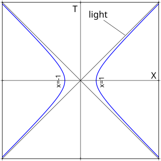
Hyperbolic motion is the motion of an object with constant proper acceleration in special relativity. It is called hyperbolic motion because the equation describing the path of the object through spacetime is a hyperbola, as can be seen when graphed on a Minkowski diagram whose coordinates represent a suitable inertial (non-accelerated) frame. This motion has several interesting features, among them that it is possible to outrun a photon if given a sufficient head start, as may be concluded from the diagram.

The Ekman spiral is an arrangement of ocean currents: the directions of horizontal current appear to twist as the depth changes. The oceanic wind driven Ekman spiral is the result of a force balance created by a shear stress force, Coriolis force and the water drag. This force balance gives a resulting current of the water different from the winds. In the ocean, there are two places where the Ekman spiral can be observed. At the surface of the ocean, the shear stress force corresponds with the wind stress force. At the bottom of the ocean, the shear stress force is created by friction with the ocean floor. This phenomenon was first observed at the surface by the Norwegian oceanographer Fridtjof Nansen during his Fram expedition. He noticed that icebergs did not drift in the same direction as the wind. His student, the Swedish oceanographer Vagn Walfrid Ekman, was the first person to physically explain this process.

An osculating circle is a circle that best approximates the curvature of a curve at a specific point. It is tangent to the curve at that point and has the same curvature as the curve at that point. The osculating circle provides a way to understand the local behavior of a curve and is commonly used in differential geometry and calculus.

The Duffing equation, named after Georg Duffing (1861–1944), is a non-linear second-order differential equation used to model certain damped and driven oscillators. The equation is given by

In algebra, the Bring radical or ultraradical of a real number a is the unique real root of the polynomial

In mathematics, parabolic cylindrical coordinates are a three-dimensional orthogonal coordinate system that results from projecting the two-dimensional parabolic coordinate system in the perpendicular -direction. Hence, the coordinate surfaces are confocal parabolic cylinders. Parabolic cylindrical coordinates have found many applications, e.g., the potential theory of edges.
The derivation of the Navier–Stokes equations as well as its application and formulation for different families of fluids, is an important exercise in fluid dynamics with applications in mechanical engineering, physics, chemistry, heat transfer, and electrical engineering. A proof explaining the properties and bounds of the equations, such as Navier–Stokes existence and smoothness, is one of the important unsolved problems in mathematics.

The non-random two-liquid model is an activity coefficient model that correlates the activity coefficients of a compound with its mole fractions in the liquid phase concerned. It is frequently applied in the field of chemical engineering to calculate phase equilibria. The concept of NRTL is based on the hypothesis of Wilson that the local concentration around a molecule is different from the bulk concentration. This difference is due to a difference between the interaction energy of the central molecule with the molecules of its own kind and that with the molecules of the other kind . The energy difference also introduces a non-randomness at the local molecular level. The NRTL model belongs to the so-called local-composition models. Other models of this type are the Wilson model, the UNIQUAC model, and the group contribution model UNIFAC. These local-composition models are not thermodynamically consistent for a one-fluid model for a real mixture due to the assumption that the local composition around molecule i is independent of the local composition around molecule j. This assumption is not true, as was shown by Flemr in 1976. However, they are consistent if a hypothetical two-liquid model is used.

In mathematics, the Struve functionsHα(x), are solutions y(x) of the non-homogeneous Bessel's differential equation:
The Herschel–Bulkley fluid is a generalized model of a non-Newtonian fluid, in which the strain experienced by the fluid is related to the stress in a complicated, non-linear way. Three parameters characterize this relationship: the consistency k, the flow index n, and the yield shear stress . The consistency is a simple constant of proportionality, while the flow index measures the degree to which the fluid is shear-thinning or shear-thickening. Ordinary paint is one example of a shear-thinning fluid, while oobleck provides one realization of a shear-thickening fluid. Finally, the yield stress quantifies the amount of stress that the fluid may experience before it yields and begins to flow.
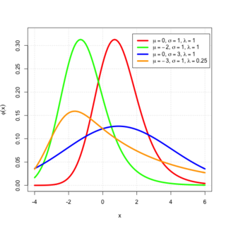
In probability theory, an exponentially modified Gaussian distribution describes the sum of independent normal and exponential random variables. An exGaussian random variable Z may be expressed as Z = X + Y, where X and Y are independent, X is Gaussian with mean μ and variance σ2, and Y is exponential of rate λ. It has a characteristic positive skew from the exponential component.

In theoretical physics, relativistic Lagrangian mechanics is Lagrangian mechanics applied in the context of special relativity and general relativity.
Accelerations in special relativity (SR) follow, as in Newtonian Mechanics, by differentiation of velocity with respect to time. Because of the Lorentz transformation and time dilation, the concepts of time and distance become more complex, which also leads to more complex definitions of "acceleration". SR as the theory of flat Minkowski spacetime remains valid in the presence of accelerations, because general relativity (GR) is only required when there is curvature of spacetime caused by the energy–momentum tensor. However, since the amount of spacetime curvature is not particularly high on Earth or its vicinity, SR remains valid for most practical purposes, such as experiments in particle accelerators.


