Delta potential

Last updated

In quantum mechanics the delta potential is a potential well mathematically described by the Dirac delta function - a generalized function. Qualitatively, it corresponds to a potential which is zero everywhere, except at a single point, where it takes an infinite value. This can be used to simulate situations where a particle is free to move in two regions of space with a barrier between the two regions. For example, an electron can move almost freely in a conducting material, but if two conducting surfaces are put close together, the interface between them acts as a barrier for the electron that can be approximated by a delta potential.

Contents

The delta potential well is a limiting case of the finite potential well, which is obtained if one maintains the product of the width of the well and the potential constant while decreasing the well's width and increasing the potential.

This article, for simplicity, only considers a one-dimensional potential well, but analysis could be expanded to more dimensions.

Single delta potential

Deltawell.png

The time-independent Schrödinger equation for the wave function ψ(x) of a particle in one dimension in a potential V(x) is

where ħ is the reduced Planck constant, and E is the energy of the particle.

The delta potential is the potential

where δ(x) is the Dirac delta function.

It is called a delta potential well if λ is negative, and a delta potential barrier if λ is positive. The delta has been defined to occur at the origin for simplicity; a shift in the delta function's argument does not change any of the following results.

Solving the Schrödinger equation

Source: [1]

The potential splits the space in two parts (x < 0 and x > 0). In each of these parts the potential is zero, and the Schrödinger equation reduces to

this is a linear differential equation with constant coefficients, whose solutions are linear combinations of eikx and eikx, where the wave number k is related to the energy by

In general, due to the presence of the delta potential in the origin, the coefficients of the solution need not be the same in both half-spaces:

where, in the case of positive energies (real k), eikx represents a wave traveling to the right, and eikx one traveling to the left.

One obtains a relation between the coefficients by imposing that the wavefunction be continuous at the origin:

A second relation can be found by studying the derivative of the wavefunction. Normally, we could also impose differentiability at the origin, but this is not possible because of the delta potential. However, if we integrate the Schrödinger equation around x = 0, over an interval [ε, +ε]:

In the limit as ε → 0, the right-hand side of this equation vanishes; the left-hand side becomes

because

Substituting the definition of ψ into this expression yields

The boundary conditions thus give the following restrictions on the coefficients

Bound state (E < 0)

The graph of the bound state wavefunction solution to the delta function potential is continuous everywhere, but its derivative is not defined at x = 0. DeltaF-WaveSolution 2.png
The graph of the bound state wavefunction solution to the delta function potential is continuous everywhere, but its derivative is not defined at x = 0.

In any one-dimensional attractive potential there will be a bound state. To find its energy, note that for E < 0, k = i2m|E|/ħ = is imaginary, and the wave functions which were oscillating for positive energies in the calculation above are now exponentially increasing or decreasing functions of x (see above). Requiring that the wave functions do not diverge at infinity eliminates half of the terms: Ar = Bl = 0. The wave function is then

From the boundary conditions and normalization conditions, it follows that

from which it follows that λ must be negative, that is, the bound state only exists for the well, and not for the barrier. The Fourier transform of this wave function is a Lorentzian function.

The energy of the bound state is then

Scattering (E > 0)

Transmission (T) and reflection (R) probability of a delta potential well. The energy E > 0 is in units of
m
l
2
2

2
{\displaystyle {\frac {m\lambda ^{2}}{2\hbar ^{2}}}}
. Dashed: classical result. Solid line: quantum mechanics. Deltapotwell.svg
Transmission (T) and reflection (R) probability of a delta potential well. The energy E > 0 is in units of . Dashed: classical result. Solid line: quantum mechanics.

For positive energies, the particle is free to move in either half-space: x < 0 or x > 0. It may be scattered at the delta-function potential.

The quantum case can be studied in the following situation: a particle incident on the barrier from the left side (Ar). It may be reflected (Al) or transmitted (Br). To find the amplitudes for reflection and transmission for incidence from the left, we put in the above equations Ar = 1 (incoming particle), Al = r (reflection), Bl = 0 (no incoming particle from the right) and Br = t (transmission), and solve for r and t even though we do not have any equations in t. The result is

Due to the mirror symmetry of the model, the amplitudes for incidence from the right are the same as those from the left. The result is that there is a non-zero probability

for the particle to be reflected. This does not depend on the sign of λ, that is, a barrier has the same probability of reflecting the particle as a well. This is a significant difference from classical mechanics, where the reflection probability would be 1 for the barrier (the particle simply bounces back), and 0 for the well (the particle passes through the well undisturbed).

The probability for transmission is

Remarks and application

The calculation presented above may at first seem unrealistic and hardly useful. However, it has proved to be a suitable model for a variety of real-life systems.

One such example regards the interfaces between two conducting materials. In the bulk of the materials, the motion of the electrons is quasi-free and can be described by the kinetic term in the above Hamiltonian with an effective mass m. Often, the surfaces of such materials are covered with oxide layers or are not ideal for other reasons. This thin, non-conducting layer may then be modeled by a local delta-function potential as above. Electrons may then tunnel from one material to the other giving rise to a current.

The operation of a scanning tunneling microscope (STM) relies on this tunneling effect. In that case, the barrier is due to the air between the tip of the STM and the underlying object. The strength of the barrier is related to the separation being stronger the further apart the two are. For a more general model of this situation, see Finite potential barrier (QM). The delta function potential barrier is the limiting case of the model considered there for very high and narrow barriers.

The above model is one-dimensional while the space around us is three-dimensional. So, in fact, one should solve the Schrödinger equation in three dimensions. On the other hand, many systems only change along one coordinate direction and are translationally invariant along the others. The Schrödinger equation may then be reduced to the case considered here by an Ansatz for the wave function of the type .

Alternatively, it is possible to generalize the delta function to exist on the surface of some domain D (see Laplacian of the indicator). [2]

The delta function model is actually a one-dimensional version of the Hydrogen atom according to the dimensional scaling method developed by the group of Dudley R. Herschbach [3] The delta function model becomes particularly useful with the double-well Dirac Delta function model which represents a one-dimensional version of the Hydrogen molecule ion, as shown in the following section.

Double delta potential

The symmetric and anti-symmetric wavefunctions for the double-well Dirac delta function model with "internuclear" distance R = 2 Doubledeltawell.png
The symmetric and anti-symmetric wavefunctions for the double-well Dirac delta function model with "internuclear" distance R = 2

The double-well Dirac delta function models a diatomic hydrogen molecule by the corresponding Schrödinger equation:

where the potential is now

where is the "internuclear" distance with Dirac delta-function (negative) peaks located at x = ±R/2 (shown in brown in the diagram). Keeping in mind the relationship of this model with its three-dimensional molecular counterpart, we use atomic units and set . Here is a formally adjustable parameter. From the single-well case, we can infer the "ansatz" for the solution to be

Matching of the wavefunction at the Dirac delta-function peaks yields the determinant

Thus, is found to be governed by the pseudo-quadratic equation

which has two solutions . For the case of equal charges (symmetric homonuclear case), λ = 1, and the pseudo-quadratic reduces to

The "+" case corresponds to a wave function symmetric about the midpoint (shown in red in the diagram), where A = B, and is called gerade . Correspondingly, the "−" case is the wave function that is anti-symmetric about the midpoint, where A = −B, and is called ungerade (shown in green in the diagram). They represent an approximation of the two lowest discrete energy states of the three-dimensional and are useful in its analysis. Analytical solutions for the energy eigenvalues for the case of symmetric charges are given by [4]

where W is the standard Lambert W function. Note that the lowest energy corresponds to the symmetric solution . In the case of unequal charges, and for that matter the three-dimensional molecular problem, the solutions are given by a generalization of the Lambert W function (see Lambert W function § Generalizations).

One of the most interesting cases is when qR  1, which results in . Thus, one has a non-trivial bound state solution with E = 0. For these specific parameters, there are many interesting properties that occur, one of which is the unusual effect that the transmission coefficient is unity at zero energy. [5]

See also

Related Research Articles

In quantum mechanics, the Hamiltonian of a system is an operator corresponding to the total energy of that system, including both kinetic energy and potential energy. Its spectrum, the system's energy spectrum or its set of energy eigenvalues, is the set of possible outcomes obtainable from a measurement of the system's total energy. Due to its close relation to the energy spectrum and time-evolution of a system, it is of fundamental importance in most formulations of quantum theory.

<span class="mw-page-title-main">Schrödinger equation</span> Description of a quantum-mechanical system

The Schrödinger equation is a linear partial differential equation that governs the wave function of a quantum-mechanical system. Its discovery was a significant landmark in the development of quantum mechanics. It is named after Erwin Schrödinger, who postulated the equation in 1925 and published it in 1926, forming the basis for the work that resulted in his Nobel Prize in Physics in 1933.

<span class="mw-page-title-main">Wave function</span> Mathematical description of the quantum state of a system

In quantum physics, a wave function is a mathematical description of the quantum state of an isolated quantum system. The most common symbols for a wave function are the Greek letters ψ and Ψ. Wave functions are complex-valued. For example, a wave function might assign a complex number to each point in a region of space. The Born rule provides the means to turn these complex probability amplitudes into actual probabilities. In one common form, it says that the squared modulus of a wave function that depends upon position is the probability density of measuring a particle as being at a given place. The integral of a wavefunction's squared modulus over all the system's degrees of freedom must be equal to 1, a condition called normalization. Since the wave function is complex-valued, only its relative phase and relative magnitude can be measured; its value does not, in isolation, tell anything about the magnitudes or directions of measurable observables. One has to apply quantum operators, whose eigenvalues correspond to sets of possible results of measurements, to the wave function ψ and calculate the statistical distributions for measurable quantities.

<span class="mw-page-title-main">Noether's theorem</span> Statement relating differentiable symmetries to conserved quantities

Noether's theorem states that every continuous symmetry of the action of a physical system with conservative forces has a corresponding conservation law. This is the first of two theorems proven by mathematician Emmy Noether in 1915 and published in 1918. The action of a physical system is the integral over time of a Lagrangian function, from which the system's behavior can be determined by the principle of least action. This theorem only applies to continuous and smooth symmetries of physical space.

<span class="mw-page-title-main">Ground state</span> Lowest energy level of a quantum system

The ground state of a quantum-mechanical system is its stationary state of lowest energy; the energy of the ground state is known as the zero-point energy of the system. An excited state is any state with energy greater than the ground state. In quantum field theory, the ground state is usually called the vacuum state or the vacuum.

<span class="mw-page-title-main">Bloch's theorem</span> Fundamental theorem in condensed matter physics

In condensed matter physics, Bloch's theorem states that solutions to the Schrödinger equation in a periodic potential can be expressed as plane waves modulated by periodic functions. The theorem is named after the Swiss physicist Felix Bloch, who discovered the theorem in 1929. Mathematically, they are written

<span class="mw-page-title-main">Path integral formulation</span> Formulation of quantum mechanics

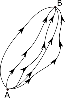
The path integral formulation is a description in quantum mechanics that generalizes the stationary action principle of classical mechanics. It replaces the classical notion of a single, unique classical trajectory for a system with a sum, or functional integral, over an infinity of quantum-mechanically possible trajectories to compute a quantum amplitude.

In mathematical physics, the WKB approximation or WKB method is a method for finding approximate solutions to linear differential equations with spatially varying coefficients. It is typically used for a semiclassical calculation in quantum mechanics in which the wavefunction is recast as an exponential function, semiclassically expanded, and then either the amplitude or the phase is taken to be changing slowly.

In quantum mechanics, the canonical commutation relation is the fundamental relation between canonical conjugate quantities. For example,

The Compton wavelength is a quantum mechanical property of a particle, defined as the wavelength of a photon the energy of which is the same as the rest energy of that particle. It was introduced by Arthur Compton in 1923 in his explanation of the scattering of photons by electrons.

In quantum mechanics, the momentum operator is the operator associated with the linear momentum. The momentum operator is, in the position representation, an example of a differential operator. For the case of one particle in one spatial dimension, the definition is:

<span class="mw-page-title-main">Degenerate energy levels</span> Energy level of a quantum system that corresponds to two or more different measurable states

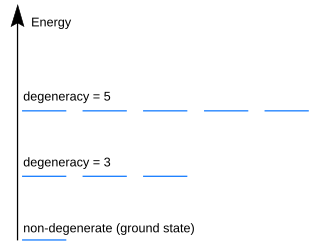
In quantum mechanics, an energy level is degenerate if it corresponds to two or more different measurable states of a quantum system. Conversely, two or more different states of a quantum mechanical system are said to be degenerate if they give the same value of energy upon measurement. The number of different states corresponding to a particular energy level is known as the degree of degeneracy of the level. It is represented mathematically by the Hamiltonian for the system having more than one linearly independent eigenstate with the same energy eigenvalue. When this is the case, energy alone is not enough to characterize what state the system is in, and other quantum numbers are needed to characterize the exact state when distinction is desired. In classical mechanics, this can be understood in terms of different possible trajectories corresponding to the same energy.

<span class="mw-page-title-main">Charge density</span> Electric charge per unit length, area or volume

In electromagnetism, charge density is the amount of electric charge per unit length, surface area, or volume. Volume charge density is the quantity of charge per unit volume, measured in the SI system in coulombs per cubic meter (C⋅m−3), at any point in a volume. Surface charge density (σ) is the quantity of charge per unit area, measured in coulombs per square meter (C⋅m−2), at any point on a surface charge distribution on a two dimensional surface. Linear charge density (λ) is the quantity of charge per unit length, measured in coulombs per meter (C⋅m−1), at any point on a line charge distribution. Charge density can be either positive or negative, since electric charge can be either positive or negative.

In solid-state physics, the nearly free electron model is a quantum mechanical model of physical properties of electrons that can move almost freely through the crystal lattice of a solid. The model is closely related to the more conceptual empty lattice approximation. The model enables understanding and calculation of the electronic band structures, especially of metals.

The Newman–Penrose (NP) formalism is a set of notation developed by Ezra T. Newman and Roger Penrose for general relativity (GR). Their notation is an effort to treat general relativity in terms of spinor notation, which introduces complex forms of the usual variables used in GR. The NP formalism is itself a special case of the tetrad formalism, where the tensors of the theory are projected onto a complete vector basis at each point in spacetime. Usually this vector basis is chosen to reflect some symmetry of the spacetime, leading to simplified expressions for physical observables. In the case of the NP formalism, the vector basis chosen is a null tetrad: a set of four null vectors—two real, and a complex-conjugate pair. The two real members often asymptotically point radially inward and radially outward, and the formalism is well adapted to treatment of the propagation of radiation in curved spacetime. The Weyl scalars, derived from the Weyl tensor, are often used. In particular, it can be shown that one of these scalars— in the appropriate frame—encodes the outgoing gravitational radiation of an asymptotically flat system.

The Gamow factor, Sommerfeld factor or Gamow–Sommerfeld factor, named after its discoverer George Gamow or after Arnold Sommerfeld, is a probability factor for two nuclear particles' chance of overcoming the Coulomb barrier in order to undergo nuclear reactions, for example in nuclear fusion. By classical physics, there is almost no possibility for protons to fuse by crossing each other's Coulomb barrier at temperatures commonly observed to cause fusion, such as those found in the sun. When George Gamow instead applied quantum mechanics to the problem, he found that there was a significant chance for the fusion due to tunneling.

This article relates the Schrödinger equation with the path integral formulation of quantum mechanics using a simple nonrelativistic one-dimensional single-particle Hamiltonian composed of kinetic and potential energy.

An LC circuit can be quantized using the same methods as for the quantum harmonic oscillator. An LC circuit is a variety of resonant circuit, and consists of an inductor, represented by the letter L, and a capacitor, represented by the letter C. When connected together, an electric current can alternate between them at the circuit's resonant frequency:

The quantum cylindrical quadrupole is a solution to the Schrödinger equation, where is the reduced Planck constant, is the mass of the particle, is the imaginary unit and is time.

<span class="mw-page-title-main">Two-body Dirac equations</span> Quantum field theory equations

In quantum field theory, and in the significant subfields of quantum electrodynamics (QED) and quantum chromodynamics (QCD), the two-body Dirac equations (TBDE) of constraint dynamics provide a three-dimensional yet manifestly covariant reformulation of the Bethe–Salpeter equation for two spin-1/2 particles. Such a reformulation is necessary since without it, as shown by Nakanishi, the Bethe–Salpeter equation possesses negative-norm solutions arising from the presence of an essentially relativistic degree of freedom, the relative time. These "ghost" states have spoiled the naive interpretation of the Bethe–Salpeter equation as a quantum mechanical wave equation. The two-body Dirac equations of constraint dynamics rectify this flaw. The forms of these equations can not only be derived from quantum field theory they can also be derived purely in the context of Dirac's constraint dynamics and relativistic mechanics and quantum mechanics. Their structures, unlike the more familiar two-body Dirac equation of Breit, which is a single equation, are that of two simultaneous quantum relativistic wave equations. A single two-body Dirac equation similar to the Breit equation can be derived from the TBDE. Unlike the Breit equation, it is manifestly covariant and free from the types of singularities that prevent a strictly nonperturbative treatment of the Breit equation. In applications of the TBDE to QED, the two particles interact by way of four-vector potentials derived from the field theoretic electromagnetic interactions between the two particles. In applications to QCD, the two particles interact by way of four-vector potentials and Lorentz invariant scalar interactions, derived in part from the field theoretic chromomagnetic interactions between the quarks and in part by phenomenological considerations. As with the Breit equation a sixteen-component spinor Ψ is used.

References

  1. "quantum mechanics - Wave function with a delta potential". Physics Stack Exchange. Retrieved 2021-03-29.
  2. Lange, Rutger-Jan (2012), "Potential theory, path integrals and the Laplacian of the indicator", Journal of High Energy Physics, 2012 (11): 1–49, arXiv: 1302.0864 , Bibcode:2012JHEP...11..032L, doi:10.1007/JHEP11(2012)032, S2CID   56188533
  3. D.R. Herschbach, J.S. Avery, and O. Goscinski (eds.), Dimensional Scaling in Chemical Physics, Springer, (1992).
  4. T. C. Scott, J. F. Babb, A. Dalgarno and John D. Morgan III, "The Calculation of Exchange Forces: General Results and Specific Models", J. Chem. Phys., 99, pp. 2841–2854, (1993).
  5. van Dijk, W.; Kiers, K. A. (1992). "Time delay in simple one‐dimensional systems". American Journal of Physics. 60 (6). American Association of Physics Teachers (AAPT): 520–527. Bibcode:1992AmJPh..60..520V. doi:10.1119/1.16866. ISSN   0002-9505.