Elementary effects method

Last updated

Published in 1991 by Max Morris [1] the elementary effects (EE) method [2] is one of the most used [3] [4] [5] [6] screening methods in sensitivity analysis.

EE is applied to identify non-influential inputs for a computationally costly mathematical model or for a model with a large number of inputs, where the costs of estimating other sensitivity analysis measures such as the variance-based measures is not affordable. Like all screening, the EE method provides qualitative sensitivity analysis measures, i.e. measures which allow the identification of non-influential inputs or which allow to rank the input factors in order of importance, but do not quantify exactly the relative importance of the inputs.

Methodology

To exemplify the EE method, let us assume to consider a mathematical model with input factors. Let be the output of interest (a scalar for simplicity):

The original EE method of Morris [2] provides two sensitivity measures for each input factor:

These two measures are obtained through a design based on the construction of a series of trajectories in the space of the inputs, where inputs are randomly moved One-At-a-Time (OAT). In this design, each model input is assumed to vary across selected levels in the space of the input factors. The region of experimentation is thus a -dimensional -level grid.

Each trajectory is composed of points since input factors move one by one of a step in while all the others remain fixed.

Along each trajectory the so-called elementary effect for each input factor is defined as:

,

where is any selected value in such that the transformed point is still in for each index

elementary effects are estimated for each input by randomly sampling points .

Usually ~ 4-10, depending on the number of input factors, on the computational cost of the model and on the choice of the number of levels , since a high number of levels to be explored needs to be balanced by a high number of trajectories, in order to obtain an exploratory sample. It is demonstrated that a convenient choice for the parameters and is even and equal to , as this ensures equal probability of sampling in the input space.

In case input factors are not uniformly distributed, the best practice is to sample in the space of the quantiles and to obtain the inputs values using inverse cumulative distribution functions. Note that in this case equals the step taken by the inputs in the space of the quantiles.

The two measures and are defined as the mean and the standard deviation of the distribution of the elementary effects of each input:

,
.

These two measures need to be read together (e.g. on a two-dimensional graph) in order to rank input factors in order of importance and identify those inputs which do not influence the output variability. Low values of both and correspond to a non-influent input.

An improvement of this method was developed by Campolongo et al. [7] who proposed a revised measure , which on its own is sufficient to provide a reliable ranking of the input factors. The revised measure is the mean of the distribution of the absolute values of the elementary effects of the input factors:

.

The use of solves the problem of the effects of opposite signs which occurs when the model is non-monotonic and which can cancel each other out, thus resulting in a low value for .

An efficient technical scheme to construct the trajectories used in the EE method is presented in the original paper by Morris while an improvement strategy aimed at better exploring the input space is proposed by Campolongo et al..

Related Research Articles

<span class="mw-page-title-main">Feynman diagram</span> Pictorial representation of the behavior of subatomic particles

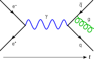
In theoretical physics, a Feynman diagram is a pictorial representation of the mathematical expressions describing the behavior and interaction of subatomic particles. The scheme is named after American physicist Richard Feynman, who introduced the diagrams in 1948. The interaction of subatomic particles can be complex and difficult to understand; Feynman diagrams give a simple visualization of what would otherwise be an arcane and abstract formula. According to David Kaiser, "Since the middle of the 20th century, theoretical physicists have increasingly turned to this tool to help them undertake critical calculations. Feynman diagrams have revolutionized nearly every aspect of theoretical physics." While the diagrams are applied primarily to quantum field theory, they can also be used in other areas of physics, such as solid-state theory. Frank Wilczek wrote that the calculations that won him the 2004 Nobel Prize in Physics "would have been literally unthinkable without Feynman diagrams, as would [Wilczek's] calculations that established a route to production and observation of the Higgs particle."

<span class="mw-page-title-main">Entropy (information theory)</span> Expected amount of information needed to specify the output of a stochastic data source

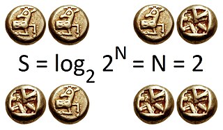
In information theory, the entropy of a random variable is the average level of "information", "surprise", or "uncertainty" inherent to the variable's possible outcomes. Given a discrete random variable , which takes values in the alphabet and is distributed according to :

In probability theory, the central limit theorem (CLT) states that, under appropriate conditions, the distribution of a normalized version of the sample mean converges to a standard normal distribution. This holds even if the original variables themselves are not normally distributed. There are several versions of the CLT, each applying in the context of different conditions.

In mathematical analysis, the Haar measure assigns an "invariant volume" to subsets of locally compact topological groups, consequently defining an integral for functions on those groups.

In statistics, maximum likelihood estimation (MLE) is a method of estimating the parameters of an assumed probability distribution, given some observed data. This is achieved by maximizing a likelihood function so that, under the assumed statistical model, the observed data is most probable. The point in the parameter space that maximizes the likelihood function is called the maximum likelihood estimate. The logic of maximum likelihood is both intuitive and flexible, and as such the method has become a dominant means of statistical inference.

In mathematics, the Kronecker delta is a function of two variables, usually just non-negative integers. The function is 1 if the variables are equal, and 0 otherwise:

In calculus and real analysis, absolute continuity is a smoothness property of functions that is stronger than continuity and uniform continuity. The notion of absolute continuity allows one to obtain generalizations of the relationship between the two central operations of calculus—differentiation and integration. This relationship is commonly characterized in the framework of Riemann integration, but with absolute continuity it may be formulated in terms of Lebesgue integration. For real-valued functions on the real line, two interrelated notions appear: absolute continuity of functions and absolute continuity of measures. These two notions are generalized in different directions. The usual derivative of a function is related to the Radon–Nikodym derivative, or density, of a measure. We have the following chains of inclusions for functions over a compact subset of the real line:

In the calculus of variations and classical mechanics, the Euler–Lagrange equations are a system of second-order ordinary differential equations whose solutions are stationary points of the given action functional. The equations were discovered in the 1750s by Swiss mathematician Leonhard Euler and Italian mathematician Joseph-Louis Lagrange.

In the mathematical field of measure theory, an outer measure or exterior measure is a function defined on all subsets of a given set with values in the extended real numbers satisfying some additional technical conditions. The theory of outer measures was first introduced by Constantin Carathéodory to provide an abstract basis for the theory of measurable sets and countably additive measures. Carathéodory's work on outer measures found many applications in measure-theoretic set theory, and was used in an essential way by Hausdorff to define a dimension-like metric invariant now called Hausdorff dimension. Outer measures are commonly used in the field of geometric measure theory.

In information geometry, the Fisher information metric is a particular Riemannian metric which can be defined on a smooth statistical manifold, i.e., a smooth manifold whose points are probability measures defined on a common probability space. It can be used to calculate the informational difference between measurements.

In physics, the Hamilton–Jacobi equation, named after William Rowan Hamilton and Carl Gustav Jacob Jacobi, is an alternative formulation of classical mechanics, equivalent to other formulations such as Newton's laws of motion, Lagrangian mechanics and Hamiltonian mechanics.

In mathematics, differential algebra is, broadly speaking, the area of mathematics consisting in the study of differential equations and differential operators as algebraic objects in view of deriving properties of differential equations and operators without computing the solutions, similarly as polynomial algebras are used for the study of algebraic varieties, which are solution sets of systems of polynomial equations. Weyl algebras and Lie algebras may be considered as belonging to differential algebra.

In statistics and probability theory, a point process or point field is a collection of mathematical points randomly located on a mathematical space such as the real line or Euclidean space. Point processes can be used for spatial data analysis, which is of interest in such diverse disciplines as forestry, plant ecology, epidemiology, geography, seismology, materials science, astronomy, telecommunications, computational neuroscience, economics and others.

Differential entropy is a concept in information theory that began as an attempt by Claude Shannon to extend the idea of (Shannon) entropy, a measure of average (surprisal) of a random variable, to continuous probability distributions. Unfortunately, Shannon did not derive this formula, and rather just assumed it was the correct continuous analogue of discrete entropy, but it is not. The actual continuous version of discrete entropy is the limiting density of discrete points (LDDP). Differential entropy is commonly encountered in the literature, but it is a limiting case of the LDDP, and one that loses its fundamental association with discrete entropy.

In mathematics, a Bose–Mesner algebra is a special set of matrices which arise from a combinatorial structure known as an association scheme, together with the usual set of rules for combining those matrices, such that they form an associative algebra, or, more precisely, a unitary commutative algebra. Among these rules are:

Statistical Football prediction is a method used in sports betting, to predict the outcome of football matches by means of statistical tools. The goal of statistical match prediction is to outperform the predictions of bookmakers, who use them to set odds on the outcome of football matches.

In applied statistics, the Morris method for global sensitivity analysis is a so-called one-step-at-a-time method, meaning that in each run only one input parameter is given a new value. It facilitates a global sensitivity analysis by making a number r of local changes at different points x(1 → r) of the possible range of input values.

In statistical mechanics, the mean squared displacement is a measure of the deviation of the position of a particle with respect to a reference position over time. It is the most common measure of the spatial extent of random motion, and can be thought of as measuring the portion of the system "explored" by the random walker. In the realm of biophysics and environmental engineering, the Mean Squared Displacement is measured over time to determine if a particle is spreading slowly due to diffusion, or if an advective force is also contributing. Another relevant concept, the variance-related diameter, is also used in studying the transportation and mixing phenomena in the realm of environmental engineering. It prominently appears in the Debye–Waller factor and in the Langevin equation.

A partially linear model is a form of semiparametric model, since it contains parametric and nonparametric elements. Application of the least squares estimators is available to partially linear model, if the hypothesis of the known of nonparametric element is valid. Partially linear equations were first used in the analysis of the relationship between temperature and usage of electricity by Engle, Granger, Rice and Weiss (1986). Typical application of partially linear model in the field of Microeconomics is presented by Tripathi in the case of profitability of firm's production in 1997. Also, partially linear model applied successfully in some other academic field. In 1994, Zeger and Diggle introduced partially linear model into biometrics. In environmental science, Parda-Sanchez et al. used partially linear model to analysis collected data in 2000. So far, partially linear model was optimized in many other statistic methods. In 1988, Robinson applied Nadaraya-Waston kernel estimator to test the nonparametric element to build a least-squares estimator After that, in 1997, local linear method was found by Truong.

In mathematics, the hypergraph regularity method is a powerful tool in extremal graph theory that refers to the combined application of the hypergraph regularity lemma and the associated counting lemma. It is a generalization of the graph regularity method, which refers to the use of Szemerédi's regularity and counting lemmas.

References

  1. https://www.stat.iastate.edu/people/max-morris Home Page of Max D. Morris at Iowa State University
  2. 1 2 Morris, M. D. (1991). Factorial sampling plans for preliminary computational experiments. Technometrics, 33, 161–174.
  3. Borgonovo, Emanuele, and Elmar Plischke. 2016. “Sensitivity Analysis: A Review of Recent Advances.” European Journal of Operational Research 248 (3): 869–87. https://doi.org/10.1016/J.EJOR.2015.06.032.
  4. Iooss, Bertrand, and Paul Lemaître. 2015. “A Review on Global Sensitivity Analysis Methods.” In Uncertainty Management in Simulation-Optimization of Complex Systems, edited by G. Dellino and C. Meloni, 101–22. Boston, MA: Springer, Boston, MA. https://doi.org/10.1007/978-1-4899-7547-8_5.
  5. Norton, J.P. 2015. “An Introduction to Sensitivity Assessment of Simulation Models.” Environmental Modelling & Software 69 (C): 166–74. https://doi.org/10.1016/j.envsoft.2015.03.020.
  6. Wei, Pengfei, Zhenzhou Lu, and Jingwen Song. 2015. “Variable Importance Analysis: A Comprehensive Review.” Reliability Engineering & System Safety 142: 399–432. https://doi.org/10.1016/j.ress.2015.05.018.
  7. Campolongo, F., J. Cariboni, and A. Saltelli (2007). An effective screening design for sensitivity analysis of large models. Environmental Modelling and Software, 22, 15091518.