Sensitivity analysis

Sensitivity analysis is the study of how the uncertainty in the output of a mathematical model or system (numerical or otherwise) can be divided and allocated to different sources of uncertainty in its inputs. A related practice is uncertainty analysis, which has a greater focus on uncertainty quantification and propagation of uncertainty; ideally, uncertainty and sensitivity analysis should be run in tandem.

The process of recalculating outcomes under alternative assumptions to determine the impact of a variable under sensitivity analysis can be useful for a range of purposes, ^[1] including:

• Testing the robustness of the results of a model or system in the presence of uncertainty.
• Increased understanding of the relationships between input and output variables in a system or model.
• Uncertainty reduction, through the identification of model input that cause significant uncertainty in the output and should therefore be the focus of attention in order to increase robustness (perhaps by further research).
• Searching for errors in the model (by encountering unexpected relationships between inputs and outputs).
• Model simplification – fixing model input that has no effect on the output, or identifying and removing redundant parts of the model structure.
• Enhancing communication from modelers to decision makers (e.g. by making recommendations more credible, understandable, compelling or persuasive).
• Finding regions in the space of input factors for which the model output is either maximum or minimum or meets some optimum criterion (see optimization and Monte Carlo filtering).
• In case of calibrating models with large number of parameters, a primary sensitivity test can ease the calibration stage by focusing on the sensitive parameters. Not knowing the sensitivity of parameters can result in time being uselessly spent on non-sensitive ones. ^[2]
• To seek to identify important connections between observations, model inputs, and predictions or forecasts, leading to the development of better models. ^{[3] [4]}

Overview

A mathematical model (for example in biology, climate change, economics, or engineering) can be highly complex, and as a result, its relationships between inputs and outputs may be poorly understood. In such cases, the model can be viewed as a black box, i.e. the output is an "opaque" function of its inputs. Quite often, some or all of the model inputs are subject to sources of uncertainty, including errors of measurement, absence of information and poor or partial understanding of the driving forces and mechanisms. This uncertainty imposes a limit on our confidence in the response or output of the model. Further, models may have to cope with the natural intrinsic variability of the system (aleatory), such as the occurrence of stochastic events. ^[5]

In models involving many input variables, sensitivity analysis is an essential ingredient of model building and quality assurance. National and international agencies involved in impact assessment studies have included sections devoted to sensitivity analysis in their guidelines. Examples are the European Commission (see e.g. the guidelines for impact assessment), ^[6] the White House Office of Management and Budget, the Intergovernmental Panel on Climate Change and US Environmental Protection Agency's modeling guidelines. ^[7]

Settings, constraints, and related issues

Settings and constraints

The choice of method of sensitivity analysis is typically dictated by a number of problem constraints or settings. Some of the most common are

• Computational expense: Sensitivity analysis is almost always performed by running the model a (possibly large) number of times, i.e. a sampling-based approach. ^[8] This can be a significant problem when,
  • A single run of the model takes a significant amount of time (minutes, hours or longer). This is not unusual with very complex models.
  • The model has a large number of uncertain inputs. Sensitivity analysis is essentially the exploration of the multidimensional input space, which grows exponentially in size with the number of inputs. See the curse of dimensionality.

Computational expense is a problem in many practical sensitivity analyses. Some methods of reducing computational expense include the use of emulators (for large models), and screening methods (for reducing the dimensionality of the problem). Another method is to use an event-based sensitivity analysis method for variable selection for time-constrained applications. ^[9] This is an input variable selection (IVS) method that assembles together information about the trace of the changes in system inputs and outputs using sensitivity analysis to produce an input/output trigger/event matrix that is designed to map the relationships between input data as causes that trigger events and the output data that describes the actual events. The cause-effect relationship between the causes of state change i.e. input variables and the effect system output parameters determines which set of inputs have a genuine impact on a given output. The method has a clear advantage over analytical and computational IVS method since it tries to understand and interpret system state change in the shortest possible time with minimum computational overhead. ^{[9] [10]}

• Correlated inputs: Most common sensitivity analysis methods assume independence between model inputs, but sometimes inputs can be strongly correlated. This is still an immature field of research and definitive methods have yet to be established.
• Nonlinearity: Some sensitivity analysis approaches, such as those based on linear regression, can inaccurately measure sensitivity when the model response is nonlinear with respect to its inputs. In such cases, variance-based measures are more appropriate.
• Multiple outputs: Virtually all sensitivity analysis methods consider a single univariate model output, yet many models output a large number of possibly spatially or time-dependent data. Note that this does not preclude the possibility of performing different sensitivity analyses for each output of interest. However, for models in which the outputs are correlated, the sensitivity measures can be hard to interpret.

Assumptions vs. inferences

In uncertainty and sensitivity analysis there is a crucial trade off between how scrupulous an analyst is in exploring the input assumptions and how wide the resulting inference may be. The point is well illustrated by the econometrician Edward E. Leamer: ^{[11] [12]}

I have proposed a form of organized sensitivity analysis that I call 'global sensitivity analysis' in which a neighborhood of alternative assumptions is selected and the corresponding interval of inferences is identified. Conclusions are judged to be sturdy only if the neighborhood of assumptions is wide enough to be credible and the corresponding interval of inferences is narrow enough to be useful.

Note Leamer's emphasis is on the need for 'credibility' in the selection of assumptions. The easiest way to invalidate a model is to demonstrate that it is fragile with respect to the uncertainty in the assumptions or to show that its assumptions have not been taken 'wide enough'. The same concept is expressed by Jerome R. Ravetz, for whom bad modeling is when uncertainties in inputs must be suppressed lest outputs become indeterminate. ^[13]

Pitfalls and difficulties

Some common difficulties in sensitivity analysis include

• Too many model inputs to analyse. Screening can be used to reduce dimensionality. Another way to tackle the curse of dimensionality is to use sampling based on low discrepancy sequences ^[14]
• The model takes too long to run. Emulators (including HDMR) can reduce the total time by accelerating the model or by reducing the number of model runs needed.
• There is not enough information to build probability distributions for the inputs. Probability distributions can be constructed from expert elicitation, although even then it may be hard to build distributions with great confidence. The subjectivity of the probability distributions or ranges will strongly affect the sensitivity analysis.
• Unclear purpose of the analysis. Different statistical tests and measures are applied to the problem and different factors rankings are obtained. The test should instead be tailored to the purpose of the analysis, e.g. one uses Monte Carlo filtering if one is interested in which factors are most responsible for generating high/low values of the output.
• Too many model outputs are considered. This may be acceptable for the quality assurance of sub-models but should be avoided when presenting the results of the overall analysis.
• Piecewise sensitivity. This is when one performs sensitivity analysis on one sub-model at a time. This approach is non conservative as it might overlook interactions among factors in different sub-models (Type II error).

Sensitivity analysis methods

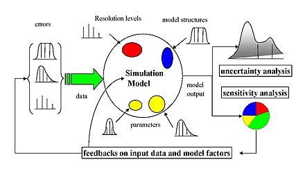
Ideal scheme of a possibly sampling-based sensitivity analysis. Uncertainty arising from different sources – errors in the data, parameter estimation procedure, alternative model structures – are propagated through the model for uncertainty analysis and their relative importance is quantified via sensitivity analysis.

Sampling-based sensitivity analysis by scatterplots. Y (vertical axis) is a function of four factors. The points in the four scatterplots are always the same though sorted differently, i.e. by Z₁, Z₂, Z₃, Z₄ in turn. Note that the abscissa is different for each plot: (−5, +5) for Z₁, (−8, +8) for Z₂, (−10, +10) for Z₃ and Z₄. Z₄ is most important in influencing Y as it imparts more 'shape' on Y.

There are a large number of approaches to performing a sensitivity analysis, many of which have been developed to address one or more of the constraints discussed above. They are also distinguished by the type of sensitivity measure, be it based on (for example) variance decompositions, partial derivatives or elementary effects. In general, however, most procedures adhere to the following outline:

1. Quantify the uncertainty in each input (e.g. ranges, probability distributions). Note that this can be difficult and many methods exist to elicit uncertainty distributions from subjective data. ^[15]
2. Identify the model output to be analysed (the target of interest should ideally have a direct relation to the problem tackled by the model).
3. Run the model a number of times using some design of experiments, ^[16] dictated by the method of choice and the input uncertainty.
4. Using the resulting model outputs, calculate the sensitivity measures of interest.

In some cases this procedure will be repeated, for example in high-dimensional problems where the user has to screen out unimportant variables before performing a full sensitivity analysis.

The various types of "core methods" (discussed below) are distinguished by the various sensitivity measures which are calculated. These categories can somehow overlap. Alternative ways of obtaining these measures, under the constraints of the problem, can be given.

One-at-a-time (OAT)

Main article: One-factor-at-a-time method

One of the simplest and most common approaches is that of changing one-factor-at-a-time (OAT), to see what effect this produces on the output. ^{[17] [18] [19]} OAT customarily involves

• moving one input variable, keeping others at their baseline (nominal) values, then,
• returning the variable to its nominal value, then repeating for each of the other inputs in the same way.

Sensitivity may then be measured by monitoring changes in the output, e.g. by partial derivatives or linear regression. This appears a logical approach as any change observed in the output will unambiguously be due to the single variable changed. Furthermore, by changing one variable at a time, one can keep all other variables fixed to their central or baseline values. This increases the comparability of the results (all 'effects' are computed with reference to the same central point in space) and minimizes the chances of computer program crashes, more likely when several input factors are changed simultaneously. OAT is frequently preferred by modelers because of practical reasons. In case of model failure under OAT analysis the modeler immediately knows which is the input factor responsible for the failure.

Despite its simplicity however, this approach does not fully explore the input space, since it does not take into account the simultaneous variation of input variables. This means that the OAT approach cannot detect the presence of interactions between input variables and is unsuitable for nonlinear models. ^[20]

The proportion of input space which remains unexplored with an OAT approach grows superexponentially with the number of inputs. For example, a 3-variable parameter space which is explored one-at-a-time is equivalent to taking points along the x, y, and z axes of a cube centered at the origin. The convex hull bounding all these points is an octahedron which has a volume only 1/6th of the total parameter space. More generally, the convex hull of the axes of a hyperrectangle forms a hyperoctahedron which has a volume fraction of ${\displaystyle 1/n!}$. With 5 inputs, the explored space already drops to less than 1% of the total parameter space. And even this is an overestimate, since the off-axis volume is not actually being sampled at all. Compare this to random sampling of the space, where the convex hull approaches the entire volume as more points are added. ^[21] While the sparsity of OAT is theoretically not a concern for linear models, true linearity is rare in nature.

Derivative-based local methods

Local derivative-based methods involve taking the partial derivative of the output Y with respect to an input factor X_i :

${\displaystyle \left|{\frac {\partial Y}{\partial X_{i}}}\right|_{{\textbf {x}}^{0}},}$

where the subscript x⁰ indicates that the derivative is taken at some fixed point in the space of the input (hence the 'local' in the name of the class). Adjoint modelling ^{[22] [23]} and Automated Differentiation ^[24] are methods which allow to compute all partial derivatives at a cost at most 4-6 times of that for evaluating the original function. Similar to OAT, local methods do not attempt to fully explore the input space, since they examine small perturbations, typically one variable at a time. It is possible to select similar samples from derivative-based sensitivity through Neural Networks and perform uncertainty quantification.

One advantage of the local methods is that it is possible to make a matrix to represent all the sensitivities in a system, thus providing an overview that cannot be achieved with global methods if there is a large number of input and output variables.

^[25]

Regression analysis

Regression analysis, in the context of sensitivity analysis, involves fitting a linear regression to the model response and using standardized regression coefficients as direct measures of sensitivity. The regression is required to be linear with respect to the data (i.e. a hyperplane, hence with no quadratic terms, etc., as regressors) because otherwise it is difficult to interpret the standardised coefficients. This method is therefore most suitable when the model response is in fact linear; linearity can be confirmed, for instance, if the coefficient of determination is large. The advantages of regression analysis are that it is simple and has a low computational cost.

Variance-based methods

Main article: Variance-based sensitivity analysis

Variance-based methods ^[26] are a class of probabilistic approaches which quantify the input and output uncertainties as probability distributions, and decompose the output variance into parts attributable to input variables and combinations of variables. The sensitivity of the output to an input variable is therefore measured by the amount of variance in the output caused by that input. These can be expressed as conditional expectations, i.e., considering a model Y = f(X) for X = {X₁, X₂, ... X_k}, a measure of sensitivity of the ith variable X_i is given as,

${\displaystyle \operatorname {Var} \left(E_{{\textbf {X}}_{\sim i}}\left(Y\mid X_{i}\right)\right)}$

where "Var" and "E" denote the variance and expected value operators respectively, and X_~i denotes the set of all input variables except X_i. This expression essentially measures the contribution X_i alone to the uncertainty (variance) in Y (averaged over variations in other variables), and is known as the first-order sensitivity index or main effect index. Importantly, it does not measure the uncertainty caused by interactions with other variables. A further measure, known as the total effect index, gives the total variance in Y caused by X_iand its interactions with any of the other input variables. Both quantities are typically standardised by dividing by Var(Y).

Variance-based methods allow full exploration of the input space, accounting for interactions, and nonlinear responses. For these reasons they are widely used when it is feasible to calculate them. Typically this calculation involves the use of Monte Carlo methods, but since this can involve many thousands of model runs, other methods (such as emulators) can be used to reduce computational expense when necessary.

Variogram analysis of response surfaces (VARS)

One of the major shortcomings of the previous sensitivity analysis methods is that none of them considers the spatially ordered structure of the response surface/output of the model Y=f(X) in the parameter space. By utilizing the concepts of directional variograms and covariograms, variogram analysis of response surfaces (VARS) addresses this weakness through recognizing a spatially continuous correlation structure to the values of Y, and hence also to the values of ${\displaystyle {\frac {\partial Y}{\partial x_{i}}}}$. ^{[27] [28]}

Basically, the higher the variability the more heterogeneous is the response surface along a particular direction/parameter, at a specific perturbation scale. Accordingly, in the VARS framework, the values of directional variograms for a given perturbation scale can be considered as a comprehensive illustration of sensitivity information, through linking variogram analysis to both direction and perturbation scale concepts. As a result, the VARS framework accounts for the fact that sensitivity is a scale-dependent concept, and thus overcomes the scale issue of traditional sensitivity analysis methods. ^[29] More importantly, VARS is able to provide relatively stable and statistically robust estimates of parameter sensitivity with much lower computational cost than other strategies (about two orders of magnitude more efficient). ^[30] Noteworthy, it has been shown that there is a theoretical link between the VARS framework and the variance-based and derivative-based approaches.

Alternative methods

A number of methods have been developed to overcome some of the constraints discussed above, which would otherwise make the estimation of sensitivity measures infeasible (most often due to computational expense). Generally, these methods focus on efficiently calculating variance-based measures of sensitivity.

Emulators

Emulators (also known as metamodels, surrogate models or response surfaces) are data-modeling/machine learning approaches that involve building a relatively simple mathematical function, known as an emulator, that approximates the input/output behavior of the model itself. ^[31] In other words, it is the concept of "modeling a model" (hence the name "metamodel"). The idea is that, although computer models may be a very complex series of equations that can take a long time to solve, they can always be regarded as a function of their inputs Y = f(X). By running the model at a number of points in the input space, it may be possible to fit a much simpler emulator η(X), such that η(X) ≈ f(X) to within an acceptable margin of error. ^[32] Then, sensitivity measures can be calculated from the emulator (either with Monte Carlo or analytically), which will have a negligible additional computational cost. Importantly, the number of model runs required to fit the emulator can be orders of magnitude less than the number of runs required to directly estimate the sensitivity measures from the model. ^[33]

Clearly, the crux of an emulator approach is to find an η (emulator) that is a sufficiently close approximation to the model f. This requires the following steps,

1. Sampling (running) the model at a number of points in its input space. This requires a sample design.
2. Selecting a type of emulator (mathematical function) to use.
3. "Training" the emulator using the sample data from the model – this generally involves adjusting the emulator parameters until the emulator mimics the true model as well as possible.

Sampling the model can often be done with low-discrepancy sequences, such as the Sobol sequence – due to mathematician Ilya M. Sobol or Latin hypercube sampling, although random designs can also be used, at the loss of some efficiency. The selection of the emulator type and the training are intrinsically linked since the training method will be dependent on the class of emulator. Some types of emulators that have been used successfully for sensitivity analysis include,

• Gaussian processes ^[33] (also known as kriging), where any combination of output points is assumed to be distributed as a multivariate Gaussian distribution. Recently, "treed" Gaussian processes have been used to deal with heteroscedastic and discontinuous responses. ^{[34] [35]}
• Random forests, ^[31] in which a large number of decision trees are trained, and the result averaged.
• Gradient boosting, ^[31] where a succession of simple regressions are used to weight data points to sequentially reduce error.
• Polynomial chaos expansions, ^[36] which use orthogonal polynomials to approximate the response surface.
• Smoothing splines, ^[37] normally used in conjunction with HDMR truncations (see below).
• Discrete Bayesian networks, ^[38] in conjunction with canonical models such as noisy models. Noisy models exploit information on the conditional independence between variables to significantly reduce dimensionality.

The use of an emulator introduces a machine learning problem, which can be difficult if the response of the model is highly nonlinear ^{[ disambiguation needed ]}. In all cases, it is useful to check the accuracy of the emulator, for example using cross-validation.

High-dimensional model representations (HDMR)

A high-dimensional model representation (HDMR) ^{[39] [40]} (the term is due to H. Rabitz ^[41] ) is essentially an emulator approach, which involves decomposing the function output into a linear combination of input terms and interactions of increasing dimensionality. The HDMR approach exploits the fact that the model can usually be well-approximated by neglecting higher-order interactions (second or third-order and above). The terms in the truncated series can then each be approximated by e.g. polynomials or splines (REFS) and the response expressed as the sum of the main effects and interactions up to the truncation order. From this perspective, HDMRs can be seen as emulators which neglect high-order interactions; the advantage is that they are able to emulate models with higher dimensionality than full-order emulators.

Fourier amplitude sensitivity test (FAST)

Main article: Fourier amplitude sensitivity testing

The Fourier amplitude sensitivity test (FAST) uses the Fourier series to represent a multivariate function (the model) in the frequency domain, using a single frequency variable. Therefore, the integrals required to calculate sensitivity indices become univariate, resulting in computational savings.

Monte Carlo filtering

Sensitivity analysis via Monte Carlo filtering ^[42] is also a sampling-based approach, whose objective is to identify regions in the space of the input factors corresponding to particular values (e.g., high or low) of the output.

Shapley effects

Shapley effects rely on Shapley values and represent the average marginal contribution of a given factors across all possible combinations of factors. These value are related to Sobol’s indices as their value falls between the first order Sobol’ effect and the total order effect. ^[43]

Applications

Examples of sensitivity analyses can be found in various area of application, such as:

• Environmental sciences
• Business
• Social sciences
• Chemistry
• Engineering
• Epidemiology
• Meta-analysis
• Multi-criteria decision making
• Time-critical decision making
• Model calibration
• Uncertainty Quantification
• Chaos theory
  • In population genetics — Whether a population will become chaotic when it receives a period of stochasticity ^{[44] : 183}

Sensitivity auditing

Main article: Sensitivity auditing

It may happen that a sensitivity analysis of a model-based study is meant to underpin an inference, and to certify its robustness, in a context where the inference feeds into a policy or decision-making process. In these cases the framing of the analysis itself, its institutional context, and the motivations of its author may become a matter of great importance, and a pure sensitivity analysis – with its emphasis on parametric uncertainty – may be seen as insufficient. The emphasis on the framing may derive inter-alia from the relevance of the policy study to different constituencies that are characterized by different norms and values, and hence by a different story about 'what the problem is' and foremost about 'who is telling the story'. Most often the framing includes more or less implicit assumptions, which could be political (e.g. which group needs to be protected) all the way to technical (e.g. which variable can be treated as a constant).

In order to take these concerns into due consideration the instruments of SA have been extended to provide an assessment of the entire knowledge and model generating process. This approach has been called 'sensitivity auditing'. It takes inspiration from NUSAP, ^[45] a method used to qualify the worth of quantitative information with the generation of `Pedigrees' of numbers. Sensitivity auditing has been especially designed for an adversarial context, where not only the nature of the evidence, but also the degree of certainty and uncertainty associated to the evidence, will be the subject of partisan interests. ^[46] Sensitivity auditing is recommended in the European Commission guidelines for impact assessment, ^[6] as well as in the report Science Advice for Policy by European Academies. ^[47]

Related concepts

Sensitivity analysis is closely related with uncertainty analysis; while the latter studies the overall uncertainty in the conclusions of the study, sensitivity analysis tries to identify what source of uncertainty weighs more on the study's conclusions.

The problem setting in sensitivity analysis also has strong similarities with the field of design of experiments. ^[48] In a design of experiments, one studies the effect of some process or intervention (the 'treatment') on some objects (the 'experimental units'). In sensitivity analysis one looks at the effect of varying the inputs of a mathematical model on the output of the model itself. In both disciplines one strives to obtain information from the system with a minimum of physical or numerical experiments.

See also

• Causality
• Elementary effects method
• Experimental uncertainty analysis
• Fourier amplitude sensitivity testing
• Info-gap decision theory
• Interval FEM
• Perturbation analysis
• Probabilistic design
• Probability bounds analysis
• Robustification
• ROC curve
• Uncertainty quantification
• Variance-based sensitivity analysis
• Multiverse analysis
• Feature selection

References

1. Pannell, D. J. (1997). "Sensitivity Analysis of Normative Economic Models: Theoretical Framework and Practical Strategies" (PDF). Agricultural Economics. 16 (2): 139–152. doi:10.1016/S0169-5150(96)01217-0 (inactive 2024-05-08).
2. Bahremand, A.; De Smedt, F. (2008). "Distributed Hydrological Modeling and Sensitivity Analysis in Torysa Watershed, Slovakia". Water Resources Management. 22 (3): 293–408. Bibcode:2008WatRM..22..393B. doi:10.1007/s11269-007-9168-x. S2CID   9710579.
3. Hill, M.; Kavetski, D.; Clark, M.; Ye, M.; Arabi, M.; Lu, D.; Foglia, L.; Mehl, S. (2015). "Practical use of computationally frugal model analysis methods". Groundwater. 54 (2): 159–170. doi: 10.1111/gwat.12330 . OSTI   1286771. PMID   25810333.
4. Hill, M.; Tiedeman, C. (2007). Effective Groundwater Model Calibration, with Analysis of Data, Sensitivities, Predictions, and Uncertainty. John Wiley & Sons.
5. Der Kiureghian, A.; Ditlevsen, O. (2009). "Aleatory or epistemic? Does it matter?". Structural Safety. 31 (2): 105–112. doi:10.1016/j.strusafe.2008.06.020.
6. European Commission. 2021. “Better Regulation Toolbox.” November 25.
7. "Archived copy" (PDF). Archived from the original (PDF) on 2011-04-26. Retrieved 2009-10-16.
8. Helton, J. C.; Johnson, J. D.; Salaberry, C. J.; Storlie, C. B. (2006). "Survey of sampling based methods for uncertainty and sensitivity analysis". Reliability Engineering and System Safety. 91 (10–11): 1175–1209. doi:10.1016/j.ress.2005.11.017.
9. Tavakoli, Siamak; Mousavi, Alireza (2013). "Event tracking for real-time unaware sensitivity analysis (EventTracker)". IEEE Transactions on Knowledge and Data Engineering. 25 (2): 348–359. doi:10.1109/tkde.2011.240. S2CID   17551372.
10. Tavakoli, Siamak; Mousavi, Alireza; Poslad, Stefan (2013). "Input variable selection in time-critical knowledge integration applications: A review, analysis, and recommendation paper". Advanced Engineering Informatics . 27 (4): 519–536. doi:10.1016/j.aei.2013.06.002.
11. Leamer, Edward E. (1983). "Let's Take the Con Out of Econometrics". American Economic Review . 73 (1): 31–43. JSTOR   1803924.
12. Leamer, Edward E. (1985). "Sensitivity Analyses Would Help". American Economic Review . 75 (3): 308–313. JSTOR   1814801.
13. Ravetz, J.R., 2007, No-Nonsense Guide to Science, New Internationalist Publications Ltd.
14. Tsvetkova, O.; Ouarda, T.B.M.J. (2019). "Quasi-Monte Carlo technique in global sensitivity analysis of wind resource assessment with a study on UAE" (PDF). Journal of Renewable and Sustainable Energy. 11 (5): 053303. doi:10.1063/1.5120035. S2CID   208835771.
15. O'Hagan, A.; et al. (2006). Uncertain Judgements: Eliciting Experts' Probabilities. Chichester: Wiley. ISBN   9780470033302.
16. Sacks, J.; Welch, W. J.; Mitchell, T. J.; Wynn, H. P. (1989). "Design and Analysis of Computer Experiments". Statistical Science. 4 (4): 409–435. doi: 10.1214/ss/1177012413 .
17. Campbell, J.; et al. (2008). "Photosynthetic Control of Atmospheric Carbonyl Sulfide During the Growing Season". Science . 322 (5904): 1085–1088. Bibcode:2008Sci...322.1085C. doi:10.1126/science.1164015. PMID   19008442. S2CID   206515456.
18. Bailis, R.; Ezzati, M.; Kammen, D. (2005). "Mortality and Greenhouse Gas Impacts of Biomass and Petroleum Energy Futures in Africa". Science . 308 (5718): 98–103. Bibcode:2005Sci...308...98B. doi:10.1126/science.1106881. PMID   15802601. S2CID   14404609.
19. Murphy, J.; et al. (2004). "Quantification of modelling uncertainties in a large ensemble of climate change simulations". Nature . 430 (7001): 768–772. Bibcode:2004Natur.430..768M. doi:10.1038/nature02771. PMID   15306806. S2CID   980153.
20. Czitrom, Veronica (1999). "One-Factor-at-a-Time Versus Designed Experiments". American Statistician. 53 (2): 126–131. doi:10.2307/2685731. JSTOR   2685731.
21. Gatzouras, D; Giannopoulos, A (2009). "Threshold for the volume spanned by random points with independent coordinates". Israel Journal of Mathematics . 169 (1): 125–153. doi: 10.1007/s11856-009-0007-z .
22. Cacuci, Dan G. Sensitivity and Uncertainty Analysis: Theory. Vol. I. Chapman & Hall.
23. Cacuci, Dan G.; Ionescu-Bujor, Mihaela; Navon, Michael (2005). Sensitivity and Uncertainty Analysis: Applications to Large-Scale Systems. Vol. II. Chapman & Hall.
24. Griewank, A. (2000). Evaluating Derivatives, Principles and Techniques of Algorithmic Differentiation. SIAM.
25. Kabir HD, Khosravi A, Nahavandi D, Nahavandi S. Uncertainty Quantification Neural Network from Similarity and Sensitivity. In2020 International Joint Conference on Neural Networks (IJCNN) 2020 Jul 19 (pp. 1-8). IEEE.
26. Sobol', I (1990). "Sensitivity estimates for nonlinear mathematical models". Matematicheskoe Modelirovanie (in Russian). 2: 112–118.; translated in English in Sobol', I (1993). "Sensitivity analysis for non-linear mathematical models". Mathematical Modeling & Computational Experiment. 1: 407–414.
27. Razavi, Saman; Gupta, Hoshin V. (January 2016). "A new framework for comprehensive, robust, and efficient global sensitivity analysis: 1. Theory". Water Resources Research. 52 (1): 423–439. Bibcode:2016WRR....52..423R. doi: 10.1002/2015WR017558 . ISSN   1944-7973.
28. Razavi, Saman; Gupta, Hoshin V. (January 2016). "A new framework for comprehensive, robust, and efficient global sensitivity analysis: 2. Application". Water Resources Research. 52 (1): 440–455. Bibcode:2016WRR....52..440R. doi: 10.1002/2015WR017559 . ISSN   1944-7973.
29. Haghnegahdar, Amin; Razavi, Saman (September 2017). "Insights into sensitivity analysis of Earth and environmental systems models: On the impact of parameter perturbation scale". Environmental Modelling & Software. 95: 115–131. Bibcode:2017EnvMS..95..115H. doi:10.1016/j.envsoft.2017.03.031.
30. Gupta, H; Razavi, S (2016). "Challenges and Future Outlook of Sensitivity Analysis". In Petropoulos, George; Srivastava, Prashant (eds.). Sensitivity Analysis in Earth Observation Modelling (1st ed.). Elsevier. pp. 397–415. ISBN   9780128030318.
31. Storlie, C.B.; Swiler, L.P.; Helton, J.C.; Sallaberry, C.J. (2009). "Implementation and evaluation of nonparametric regression procedures for sensitivity analysis of computationally demanding models". Reliability Engineering & System Safety. 94 (11): 1735–1763. doi:10.1016/j.ress.2009.05.007.
32. Wang, Shangying; Fan, Kai; Luo, Nan; Cao, Yangxiaolu; Wu, Feilun; Zhang, Carolyn; Heller, Katherine A.; You, Lingchong (2019-09-25). "Massive computational acceleration by using neural networks to emulate mechanism-based biological models". Nature Communications. 10 (1): 4354. Bibcode:2019NatCo..10.4354W. doi:10.1038/s41467-019-12342-y. ISSN   2041-1723. PMC   6761138 . PMID   31554788.
33. Oakley, J.; O'Hagan, A. (2004). "Probabilistic sensitivity analysis of complex models: a Bayesian approach". J. R. Stat. Soc. B. 66 (3): 751–769. CiteSeerX   10.1.1.6.9720 . doi:10.1111/j.1467-9868.2004.05304.x. S2CID   6130150.
34. Gramacy, R. B.; Taddy, M. A. (2010). "Categorical Inputs, Sensitivity Analysis, Optimization and Importance Tempering with tgp Version 2, an R Package for Treed Gaussian Process Models" (PDF). Journal of Statistical Software. 33 (6). doi: 10.18637/jss.v033.i06 .
35. Becker, W.; Worden, K.; Rowson, J. (2013). "Bayesian sensitivity analysis of bifurcating nonlinear models". Mechanical Systems and Signal Processing. 34 (1–2): 57–75. Bibcode:2013MSSP...34...57B. doi:10.1016/j.ymssp.2012.05.010.
36. Sudret, B. (2008). "Global sensitivity analysis using polynomial chaos expansions". Reliability Engineering & System Safety. 93 (7): 964–979. doi:10.1016/j.ress.2007.04.002.
37. Ratto, M.; Pagano, A. (2010). "Using recursive algorithms for the efficient identification of smoothing spline ANOVA models". AStA Advances in Statistical Analysis. 94 (4): 367–388. doi:10.1007/s10182-010-0148-8. S2CID   7678955.
38. Cardenas, IC (2019). "On the use of Bayesian networks as a meta-modeling approach to analyse uncertainties in slope stability analysis". Georisk: Assessment and Management of Risk for Engineered Systems and Geohazards. 13 (1): 53–65. Bibcode:2019GAMRE..13...53C. doi:10.1080/17499518.2018.1498524. S2CID   216590427.
39. Li, G.; Hu, J.; Wang, S.-W.; Georgopoulos, P.; Schoendorf, J.; Rabitz, H. (2006). "Random Sampling-High Dimensional Model Representation (RS-HDMR) and orthogonality of its different order component functions". Journal of Physical Chemistry A. 110 (7): 2474–2485. Bibcode:2006JPCA..110.2474L. doi:10.1021/jp054148m. PMID   16480307.
40. Li, G. (2002). "Practical approaches to construct RS-HDMR component functions". Journal of Physical Chemistry. 106 (37): 8721–8733. Bibcode:2002JPCA..106.8721L. doi:10.1021/jp014567t.
41. Rabitz, H (1989). "System analysis at molecular scale". Science. 246 (4927): 221–226. Bibcode:1989Sci...246..221R. doi:10.1126/science.246.4927.221. PMID   17839016. S2CID   23088466.
42. Hornberger, G.; Spear, R. (1981). "An approach to the preliminary analysis of environmental systems". Journal of Environmental Management. 7: 7–18.
43. Owen, A. B. (1 January 2014). "Sobol' Indices and Shapley Value". SIAM/ASA Journal on Uncertainty Quantification. 2 (1). Society for Industrial and Applied Mathematics: 245–251. doi:10.1137/130936233.
44. Perry, Joe; Smith, Robert; Woiwod, Ian; Morse, David (2000). Perry, Joe N; Smith, Robert H; Woiwod, Ian P; Morse, David R (eds.). Chaos in Real Data : The Analysis of Non-Linear Dynamics from Short Ecological Time Series. Population and Community Biology Series (1 ed.). Springer Science+Business Media Dordrecht. pp. xii+226. doi:10.1007/978-94-011-4010-2. ISBN   978-94-010-5772-1. S2CID   37855255.
45. Van der Sluijs, JP; Craye, M; Funtowicz, S; Kloprogge, P; Ravetz, J; Risbey, J (2005). "Combining quantitative and qualitative measures of uncertainty in model based environmental assessment: the NUSAP system". Risk Analysis. 25 (2): 481–492. Bibcode:2005RiskA..25..481V. doi:10.1111/j.1539-6924.2005.00604.x. hdl: 1874/386039 . PMID   15876219. S2CID   15988654.
46. Lo Piano, S; Robinson, M (2019). "Nutrition and public health economic evaluations under the lenses of post normal science". Futures. 112: 102436. doi:10.1016/j.futures.2019.06.008. S2CID   198636712.
47. Science Advice for Policy by European Academies, Making sense of science for policy under conditions of complexity and uncertainty, Berlin, 2019.
48. Box GEP, Hunter WG, Hunter, J. Stuart. Statistics for experimenters [Internet]. New York: Wiley & Sons

Further reading

• Cannavó, F. (2012). "Sensitivity analysis for volcanic source modeling quality assessment and model selection". Computers & Geosciences. 44: 52–59. Bibcode:2012CG.....44...52C. doi:10.1016/j.cageo.2012.03.008.
• Fassò A. (2007) "Statistical sensitivity analysis and water quality". In Wymer L. Ed, Statistical Framework for Water Quality Criteria and Monitoring. Wiley, New York.
• Fassò A., Perri P.F. (2002) "Sensitivity Analysis". In Abdel H. El-Shaarawi and Walter W. Piegorsch (eds) Encyclopedia of Environmetrics, Volume 4, pp 1968–1982, Wiley.
• Fassò A., Esposito E., Porcu E., Reverberi A.P., Vegliò F. (2003) "Statistical Sensitivity Analysis of Packed Column Reactors for Contaminated Wastewater". Environmetrics. Vol. 14, n.8, 743–759.
• Haug, Edward J.; Choi, Kyung K.; Komkov, Vadim (1986) Design sensitivity analysis of structural systems. Mathematics in Science and Engineering, 177. Academic Press, Inc., Orlando, FL.
• Pianosi, F.; Beven, K.; Freer, J.; Hall, J.W.; Rougier, J.; Stephenson, D.B.; Wagener, T. (2016). "Sensitivity analysis of environmental models: A systematic review with practical workflow". Environmental Modelling & Software. 79: 214–232. Bibcode:2016EnvMS..79..214P. doi: 10.1016/j.envsoft.2016.02.008 . hdl: 10871/21086 .
• Pilkey, O. H. and L. Pilkey-Jarvis (2007), Useless Arithmetic. Why Environmental Scientists Can't Predict the Future. New York: Columbia University Press.
• Santner, T. J.; Williams, B. J.; Notz, W.I. (2003) Design and Analysis of Computer Experiments; Springer-Verlag.
• Taleb, N. N., (2007) The Black Swan: The Impact of the Highly Improbable, Random House.

External links

• Web site with material from SAMO conference series (1995-2025)
• web-page on Sensitivity analysis – (Joint Research Centre of the European Commission)
• SimLab, the free software for global sensitivity analysis of the Joint Research Centre
• MUCM Project Archived 2013-04-24 at the Wayback Machine – Extensive resources for uncertainty and sensitivity analysis of computationally-demanding models.