An elliptic filter (also known as a Cauer filter, named after Wilhelm Cauer, or as a Zolotarev filter, after Yegor Zolotarev) is a signal processing filter with equalized ripple (equiripple) behavior in both the passband and the stopband. The amount of ripple in each band is independently adjustable, and no other filter of equal order can have a faster transition in gain between the passband and the stopband, for the given values of ripple (whether the ripple is equalized or not).[citation needed] Alternatively, one may give up the ability to adjust independently the passband and stopband ripple, and instead design a filter which is maximally insensitive to component variations.
As the ripple in the stopband approaches zero, the filter becomes a type I Chebyshev filter. As the ripple in the passband approaches zero, the filter becomes a type II Chebyshev filter and finally, as both ripple values approach zero, the filter becomes a Butterworth filter.
The gain of a lowpass elliptic filter as a function of angular frequency ω is given by:
where Rn is the nth-order elliptic rational function (sometimes known as a Chebyshev rational function) and
is the cutoff frequency
is the ripple factor
is the selectivity factor
The value of the ripple factor specifies the passband ripple, while the combination of the ripple factor and the selectivity factor specify the stopband ripple.
Properties
The frequency response of a fourth-order elliptic low-pass filter with ε=0.5 and ξ=1.05. Also shown are the minimum gain in the passband and the maximum gain in the stopband, and the transition region between normalized frequency 1 and ξA closeup of the transition region of the above plot.
In the passband, the elliptic rational function varies between zero and unity. The gain of the passband therefore will vary between 1 and .
In the stopband, the elliptic rational function varies between infinity and the discrimination factor which is defined as:
The gain of the stopband therefore will vary between 0 and .
Since the Butterworth filter is a limiting form of the Chebyshev filter, it follows that in the limit of , and such that the filter becomes a Butterworth filter
Log of the absolute value of the gain of an 8th order elliptic filter in complex frequency space (s = σ + jω) with ε = 0.5, ξ = 1.05 and ω0 = 1. The white spots are poles and the black spots are zeroes. There are a total of 16 poles and 8 double zeroes. What appears to be a single pole and zero near the transition region is actually four poles and two double zeroes as shown in the expanded view below. In this image, black corresponds to a gain of 0.0001 or less and white corresponds to a gain of 10 or more.An expanded view in the transition region of the above image, resolving the four poles and two double zeroes.
The zeroes of the gain of an elliptic filter will coincide with the poles of the elliptic rational function, which are derived in the article on elliptic rational functions.
The poles of the gain of an elliptic filter may be derived in a manner very similar to the derivation of the poles of the gain of a type I Chebyshev filter. For simplicity, assume that the cutoff frequency is equal to unity. The poles of the gain of the elliptic filter will be the zeroes of the denominator of the gain. Using the complex frequency this means that:
Defining where cd() is the Jacobi elliptic cosine function and using the definition of the elliptic rational functions yields:
where and . Solving for w
where the multiple values of the inverse cd() function are made explicit using the integer index m.
The poles of the elliptic gain function are then:
As is the case for the Chebyshev polynomials, this may be expressed in explicitly complex form (Lutovac & et al. 2001, § 12.8)
where is a function of and and are the zeroes of the elliptic rational function. is expressible for all n in terms of Jacobi elliptic functions, or algebraically for some orders, especially orders 1,2, and 3. For orders 1 and 2 we have
where
The algebraic expression for is rather involved (See Lutovac & et al. (2001, § 12.8.1)).
The nesting property of the elliptic rational functions can be used to build up higher order expressions for :
where .
Minimum order
To design an Elliptic filter using the minimum required number of elements, the minimum order of the Elliptic filter may be calculated with elliptic integrals as follows.[1] The equations account for standard low pass Elliptic filters, only. Even order modifications will introduce error that the equations do not account for.
The elliptic integral computations may eliminated with the use of the following expression.[2]
where:
and are the pass band ripple frequency and maximum ripple attenuation in dB
and are the stop band frequency and minimum stop band attenuation in dB
is the minimum number of poles, the order of the filter.
ceil[] is a round up to next integer function.
Minimum Q-factor elliptic filters
The normalized Q-factors of the poles of an 8-th order elliptic filter with ξ=1.1 as a function of ripple factor ε. Each curve represents four poles, since complex conjugate pole pairs and positive-negative pole pairs have the same Q-factor. (The blue and cyan curves nearly coincide). The Q-factor of all poles are simultaneously minimized at εQmin=1/√Ln=0.02323...
Elliptic filters are generally specified by requiring a particular value for the passband ripple, stopband ripple and the sharpness of the cutoff. This will generally specify a minimum value of the filter order which must be used. Another design consideration is the sensitivity of the gain function to the values of the electronic components used to build the filter. This sensitivity is inversely proportional to the quality factor (Q-factor) of the poles of the transfer function of the filter. The Q-factor of a pole is defined as:
and is a measure of the influence of the pole on the gain function. For an elliptic filter, it happens that, for a given order, there exists a relationship between the ripple factor and selectivity factor which simultaneously minimizes the Q-factor of all poles in the transfer function:
This results in a filter which is maximally insensitive to component variations, but the ability to independently specify the passband and stopband ripples will be lost. For such filters, as the order increases, the ripple in both bands will decrease and the rate of cutoff will increase. If one decides to use a minimum-Q elliptic filter in order to achieve a particular minimum ripple in the filter bands along with a particular rate of cutoff, the order needed will generally be greater than the order one would otherwise need without the minimum-Q restriction. An image of the absolute value of the gain will look very much like the image in the previous section, except that the poles are arranged in a circle rather than an ellipse. They will not be evenly spaced and there will be zeroes on the ω axis, unlike the Butterworth filter, whose poles are arranged in an evenly spaced circle with no zeroes.
Comparison with other linear filters
Here is an image showing the elliptic filter next to other common kind of filters obtained with the same number of coefficients:
As is clear from the image, elliptic filters are sharper than all the others, but they show ripples on the whole bandwidth.
Construction from Chebyshev transmission zeros
Elliptic filter stop bands are essentially Chebyshev filters with transmission zeros where the transmission zeros are arranged in a manner that yields an equi-ripple stop band. Given this, it is possible to convert a Chebyshev filter characteristic equation, containing the Chebyshev reflection zeros in the numerator and no transmission zeros in the denominator, to an Elliptic filter containing the Elliptic reflection zeros in the numerator and Elliptic transmission zeros in the denominator, by iteratively creating transmission zeros from the scaled inverse of the Chebyshev reflection zeros, and then reestablishing an equi-ripple Chebyshev pass band from the transmission zeros, and repeating until the iterations produce no further changes of significance to .[3] The scaling factor used, , is the stop band to pass band cutoff frequency ratios and is also known as the inverse of the "selectivity factor".[2] Since Elliptic designs are generally specified from the stop band attenuation requirements, , may be derived from the equations that establish the minimum order, n, above.
the ratio, may be derived by working the minimum order, n, problem above backwards from n to find .[2]
The characteristic polynomials, computed from and attenuation requirements, may then be translated to the transfer function polynomials, with the classic translation, where and is the pass band ripple.[3][4]
Simple example
Design an Elliptic filter with a pass band ripple of 1dB from 0 to 1 rad/sec and a stop band ripple of 40dB from at least 1.25 rad/sec to .
Applying the calculations above for the value for n prior to applying the ceil() function, n is found to be 4.83721900 rounded up to the next integer, 5, by applying the ceil() function, which means a 5 pole Elliptic filter is required to meet the specified design requirements. Applying the calculations above for needed to design a stop band of exactly 40dB of attenuation, is found to be 1.2186824.
The polynomial scaled inversion function may be performed by translating each root, s, to , which may be easily accomplished by inverting the polynomial and scaling it by , as shown.
Design a Chebyshev filters with 1dB pass band ripple.
Invert all the reflections zeros about to create transmission zeros
Create an equi-ripple pass band from the transmission zeros using the process outlined is Chebyshev transmission zeros
Repeat steps 2 and 3 until both the pass band and stop band no longer change by any appreciable amount. Typically, 15 to 25 iterations produce coefficient differences in the order of than 1.e-15.
To illustrate the steps, the below K(s) equations begin with a standard Chebyshev K(s), then iterate through the process. Visible differences are seen in the first three iterations. By time 18 iterations have been reached, the differences in K(s) become negligible. Iterations may be discontinued when the change in K(s) coefficients becomes sufficiently small so as to meet design accuracy requirements. The below K(s) iterations have all been normalized such that , however, this step may be postponed until the last iteration, if desired.
To find the transfer function, do the following.[3]
To obtain from the left half plane, factor the numerator and denominator to obtain the roots using a root finding algorithm. Discard all roots from the right half plane of the denominator, half the repeated roots in the numerator, and rebuild with the remaining roots.[3][4] Generally, normalize to 1 at .
To confirm that the example is correct, the plot of along is shown below with a pass band ripple of 1dB, a cut off frequency of 1 rad/sec, a stop band attenuation of 40dB beginning at 1.21868 rad/sec
Five pole Elliptic simulation
Even order modifications
Even order Elliptic filters implemented with passive elements, typically inductors, capacitors, and transmission lines, with terminations of equal value on each side cannot be implemented with the traditional Elliptic transfer function without the use of coupled coils, which may not be desirable or feasible. This is due to the physical inability to accommodate the even order Chebyshev reflection zeros and transmission zeros that result in the scattering matrix S12 values that exceed the S12 value at , and the finite S12 values that exist at . If it is not feasible to design the filter with one of the terminations increased or decreased to accommodate the pass band S12, then the Elliptic transfer function must be modified so as to move the lowest even order reflection zero to and the highest even order transmission zero to while maintaining the equi-ripple response of the pass band and stop band.[5]
The needed modification involves mapping each pole and zero of the Elliptic transfer function in a manner that maps the lowest frequency reflection zero to zero, the highest frequency transmission zero to , and the remaining poles and zeros as needed to maintain the equi-ripple pass band and stop band. The lowest frequency reflection zero may be found by factoring the numerator, and the highest frequency transmission zero may be found be factoring the denominator.
The translate the reflection zeros, the following equation is applied to all poles and zeros of .[5] While in theory, the translation operations may be performed on either or , the reflection zeros must be extracted from , so it is generally more efficient to perform the translation operations on .
Where:
is the original Elliptic function zero or pole
is the mapped zero or pole for the modified even order transfer function.
is the lowest frequency reflection zero in the pass band.
The sign of imaginary component of is determined by the sign of the original .
The translate the transmission zeros, the following equation is applied to all poles and zeros of .[5] While in theory, the translation operations may be performed on either or , if the reflection zeros must be extracted from , it may be more efficient to perform the translation operations on .
Where:
is the original Elliptic function zero or pole
is the mapped zero or pole for the modified even order transfer function.
is the highest frequency transmission zero in the pass band.
The sign of imaginary component of is determined by the sign of the original . If operating on the sign of the real component of must be negative to conform to the left half plane requirement.
It is important to note that all applications require both pass and stop translations. Passive network diplexers, for example, only require even order stop band translations, and perform more efficiently with untranslated even order pass bands.[5]
When is completed, an equi-ripple transfer function is created with scattering matrix values for S12 of 1 and 0 at , which may be implements with passive equally terminated networks.
The illustration below shows an 8th order Elliptic filter modified to support even order equally terminated passive networks by relocating the lowest frequency reflection zero from a finite frequency to 0 and the highest frequency transmission zero to while maintaining an equi-ripple pass band and stop band frequency response.
Even order modified Elliptic illustration
The and order computation in the Elliptic construction paragraph above are for unmodified Elliptic filters only. Although even order modifications have no effect on the pass band or stop band attenuation, small errors are to be expected in the order and computations. Therefore, it is important to apply even order modifications after all iterations complete if it is desired to preserve the pass and stop band attenuations. If the even order modified Elliptic function is created from an requirement, the actual will be slightly larger than the design . Likewise, an order, n, computation may result in a smaller value than the actual required order.
Hourglass implementation
An Hourglass filter is a special case of filter where the reflection zeros, are the reciprocal of the transmission zeros about a 3.01dB normalized cut-off attenuation frequency of 1 rad/sec, resulting all poles of the filter residing on the unit circle.[6] The Elliptic Hourglass implementation has an advantage over an Inverse Chebyshev filter in that the pass band is flatter, and has an advantage over traditional Elliptic filters in that the group delay has a less sharp peak at the cut-off frequency.
7 pole Hourglass reciprocal S11 and S12 frequency response
Syntheses process
The most straightforward way to synthesize an Hourglass filter is to design an Elliptic filter with a specified design stop band attenuation, As, and a calculated pass band attenuation that meets the lossless two-port network requirement that scattering parameters.[7] Together with the well known magnitude dB to arithmetic translation, , algebraic manipulation yields the following pass band attenuation calculated requirement.
The Ap, defined above will produce reciprocal reflection and transmission zeros about a yet unknown 3.01dB cut-off frequency. to Design an Elliptic filter with a pass band frequency of 1 rad/sec the 3.01dB attenuation frequency needs to be determined and that frequency needs to be used to inversely scale the Elliptic design polynomials. The result will be polynomials with an attenuation of 3.01dB at a normalized frequency of 1 rad/sec. Newton's method or solving the equations directly with a root finding algorithm may be used to determine the 3.01dB attenuation frequency.
Frequency scaling with Newton's method
If is the Hourglass transfer function to find the 3.01dB frequency, and is the 3dB frequency to find, the steps below may be used to find
If is not already available, multiply by to obtain .
negate all terms of when is divisible by . That would be , , , and so on. The modified function will be called , and this modification will allow the use of real numbers instead of complex numbers when evaluating the polynomial and its derivative. the real can now be used in place of the complex
Convert the desired attenuation in dB, , to a squared arithmetic gain value, , by using . For example, 3.010dB converts to 0.5, 1dB converts to 0.79432823 and so on.
Calculate the modified in Newton's method using the real value, . Always take the absolute value.
Calculate the derivative the modified with respect to the real value, . DO NOT take the absolute value of the derivative.
When steps 1) through 4) are complete, the expression involving Newton's method may be written as:
using a real value for with no complex arithmetic needed. The movement of should be limited to prevent it from going negative early in the iterations for increased reliability. When convergence is complete, can used for the that can be used to scale the original transfer function denominator. The attenuation of the modified will then be virtually the exact desired value at 1 rad/sec. If performed properly, only a handful of iterations are needed to set the attenuation through a wide range of desired attenuation values for both small and very large order filters.
Frequency scaling with root finding
Since does not contain any phase information, directly factoring the transfer function will not produce usable results. However, the transfer function may be modified by multiplying it with to eliminate all odd powers of , which in turn forces to be real at all frequencies, and then finding the frequency that result on the square of the desired attention.
If is not already available, multiply by to obtain .
Convert the desired attenuation in dB, , to a squared arithmetic gain value, , by using . For example, 3.010dB converts to 0.5, 1dB converts to 0.79432823 and so on.
Of the set of roots from above, select the positive imaginary root for all order filters, and positive real root for even order filters for .
Scaling the transfer function
When has been determined, the Hourglass transfer function polynomial may be scaled as follows:
Even order modifications
Even order Hourglass filters have the same limitations regarding equally terminated passive networks as other Elliptic filters. The same even order modifications that resolve the problem with Elliptic filters also resolve the problem with Hourglass filters.
Related Research Articles
The bilinear transform is used in digital signal processing and discrete-time control theory to transform continuous-time system representations to discrete-time and vice versa.
In engineering, a transfer function of a system, sub-system, or component is a mathematical function that models the system's output for each possible input. It is widely used in electronic engineering tools like circuit simulators and control systems. In simple cases, this function can be represented as a two-dimensional graph of an independent scalar input versus the dependent scalar output. Transfer functions for components are used to design and analyze systems assembled from components, particularly using the block diagram technique, in electronics and control theory.
In physics and electrical engineering, a cutoff frequency, corner frequency, or break frequency is a boundary in a system's frequency response at which energy flowing through the system begins to be reduced rather than passing through.
A low-pass filter is a filter that passes signals with a frequency lower than a selected cutoff frequency and attenuates signals with frequencies higher than the cutoff frequency. The exact frequency response of the filter depends on the filter design. The filter is sometimes called a high-cut filter, or treble-cut filter in audio applications. A low-pass filter is the complement of a high-pass filter.
In the mathematical field of complex analysis, elliptic functions are special kinds of meromorphic functions, that satisfy two periodicity conditions. They are named elliptic functions because they come from elliptic integrals. Those integrals are in turn named elliptic because they first were encountered for the calculation of the arc length of an ellipse.
A resistor–capacitor circuit, or RC filter or RC network, is an electric circuit composed of resistors and capacitors. It may be driven by a voltage or current source and these will produce different responses. A first order RC circuit is composed of one resistor and one capacitor and is the simplest type of RC circuit.
Chebyshev filters are analog or digital filters that have a steeper roll-off than Butterworth filters, and have either passband ripple or stopband ripple. Chebyshev filters have the property that they minimize the error between the idealized and the actual filter characteristic over the operating frequency range of the filter, but they achieve this with ripples in the passband. This type of filter is named after Pafnuty Chebyshev because its mathematical characteristics are derived from Chebyshev polynomials. Type I Chebyshev filters are usually referred to as "Chebyshev filters", while type II filters are usually called "inverse Chebyshev filters". Because of the passband ripple inherent in Chebyshev filters, filters with a smoother response in the passband but a more irregular response in the stopband are preferred for certain applications.
In signal processing, a finite impulse response (FIR) filter is a filter whose impulse response is of finite duration, because it settles to zero in finite time. This is in contrast to infinite impulse response (IIR) filters, which may have internal feedback and may continue to respond indefinitely.
The Sallen–Key topology is an electronic filter topology used to implement second-order active filters that is particularly valued for its simplicity. It is a degenerate form of a voltage-controlled voltage-source (VCVS) filter topology. It was introduced by R. P. Sallen and E. L. Key of MIT Lincoln Laboratory in 1955.
The Butterworth filter is a type of signal processing filter designed to have a frequency response that is as flat as possible in the passband. It is also referred to as a maximally flat magnitude filter. It was first described in 1930 by the British engineer and physicist Stephen Butterworth in his paper entitled "On the Theory of Filter Amplifiers".
In mathematics, a Dirac comb is a periodic function with the formula
In electronics and signal processing, a Bessel filter is a type of analog linear filter with a maximally flat group delay, which preserves the wave shape of filtered signals in the passband. Bessel filters are often used in audio crossover systems.
The Optimum "L" filter was proposed by Athanasios Papoulis in 1958. It has the maximum roll off rate for a given filter order while maintaining a monotonic frequency response. It provides a compromise between the Butterworth filter which is monotonic but has a slower roll off and the Chebyshev filter which has a faster roll off but has ripple in either the passband or stopband. The filter design is based on Legendre polynomials which is the reason for its alternate name and the "L" in Optimum "L".
Ripple in electronics is the residual periodic variation of the DC voltage within a power supply which has been derived from an alternating current (AC) source. This ripple is due to incomplete suppression of the alternating waveform after rectification. Ripple voltage originates as the output of a rectifier or from generation and commutation of DC power.
In electronics and signal processing, mainly in digital signal processing, a Gaussian filter is a filter whose impulse response is a Gaussian function. Gaussian filters have the properties of having no overshoot to a step function input while minimizing the rise and fall time. This behavior is closely connected to the fact that the Gaussian filter has the minimum possible group delay. A Gaussian filter will have the best combination of suppression of high frequencies while also minimizing spatial spread, being the critical point of the uncertainty principle. These properties are important in areas such as oscilloscopes and digital telecommunication systems.
In mathematics the elliptic rational functions are a sequence of rational functions with real coefficients. Elliptic rational functions are extensively used in the design of elliptic electronic filters..
The Mathieu equation is a linear second-order differential equation with periodic coefficients. The French mathematician, E. Léonard Mathieu, first introduced this family of differential equations, nowadays termed Mathieu equations, in his “Memoir on vibrations of an elliptic membrane” in 1868. "Mathieu functions are applicable to a wide variety of physical phenomena, e.g., diffraction, amplitude distortion, inverted pendulum, stability of a floating body, radio frequency quadrupole, and vibration in a medium with modulated density"
In thermal quantum field theory, the Matsubara frequency summation is a technique used to simplify calculations involving Euclidean path integrals.
Staggered tuning is a technique used in the design of multi-stage tuned amplifiers whereby each stage is tuned to a slightly different frequency. In comparison to synchronous tuning it produces a wider bandwidth at the expense of reduced gain. It also produces a sharper transition from the passband to the stopband. Both staggered tuning and synchronous tuning circuits are easier to tune and manufacture than many other filter types.
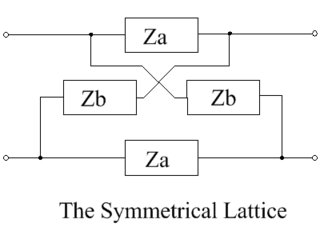
Lattice delay networks are an important subgroup of lattice networks. They are all-pass filters, so they have a flat amplitude response, but a phase response which varies linearly with frequency. All lattice circuits, regardless of their complexity, are based on the schematic shown below, which contains two series impedances, Za, and two shunt impedances, Zb. Although there is duplication of impedances in this arrangement, it offers great flexibility to the circuit designer so that, in addition to its use as delay network it can be configured to be a phase corrector, a dispersive network, an amplitude equalizer, or a low pass filter, according to the choice of components for the lattice elements.
1 2 3 Rorabaugh, C. Britton (January 1, 1993). Digital Filter Designer's Handbook (Reprinted.). Blue Ridge Summit, PA, US: Tab Books, Division of McGraw-Hill, Inc. pp.93 to 95. ISBN978-0830644315.
This page is based on this Wikipedia article Text is available under the CC BY-SA 4.0 license; additional terms may apply. Images, videos and audio are available under their respective licenses.


![The normalized Q-factors of the poles of an 8-th order elliptic filter with x = 1.1 as a function of ripple factor e. Each curve represents four poles, since complex conjugate pole pairs and positive-negative pole pairs have the same Q-factor. (The blue and cyan curves nearly coincide). The Q-factor of all poles are simultaneously minimized at eQmin = 1 / [?]Ln = 0.02323... Elliptic8 Qfactor.png](http://upload.wikimedia.org/wikipedia/commons/thumb/7/73/Elliptic8_Qfactor.png/400px-Elliptic8_Qfactor.png)