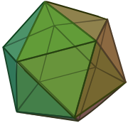
 An icosahedron.
 A highly divided geodesic polyhedron based on the icosahedron.
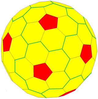
 A highly divided Goldberg polyhedron; the dual of the previous image.

A geodesic grid is a spatial grid based on a geodesic polyhedron or Goldberg polyhedron.
A geodesic grid is a spatial grid based on a geodesic polyhedron or Goldberg polyhedron.
The earliest use of the (icosahedral) geodesic grid in geophysical modeling dates back to 1968 and the work by Sadourny, Arakawa, and Mintz [1] and Williamson. [2] [3] Later work expanded on this base. [4] [5] [6] [7] [8]
A geodesic grid is a global Earth reference that uses triangular tiles based on the subdivision of a polyhedron (usually the icosahedron, and usually a Class I subdivision) to subdivide the surface of the Earth. Such a grid does not have a straightforward relationship to latitude and longitude, but conforms to many of the main criteria for a statistically valid discrete global grid. [9] Primarily, the cells' area and shape are generally similar, especially near the poles where many other spatial grids have singularities or heavy distortion. The popular Quaternary Triangular Mesh (QTM) falls into this category. [10]
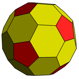
Geodesic grids may use the dual polyhedron of the geodesic polyhedron, which is the Goldberg polyhedron. Goldberg polyhedra are made up of hexagons and (if based on the icosahedron) 12 pentagons. One implementation that uses an icosahedron as the base polyhedron, hexagonal cells, and the Snyder equal-area projection is known as the Icosahedron Snyder Equal Area (ISEA) grid. [11]


In biodiversity science, geodesic grids are a global extension of local discrete grids that are staked out in field studies to ensure appropriate statistical sampling and larger multi-use grids deployed at regional and national levels to develop an aggregated understanding of biodiversity. These grids translate environmental and ecological monitoring data from multiple spatial and temporal scales into assessments of current ecological condition and forecasts of risks to our natural resources. A geodesic grid allows local to global assimilation of ecologically significant information at its own level of granularity. [13]
When modeling the weather, ocean circulation, or the climate, partial differential equations are used to describe the evolution of these systems over time. Because computer programs are used to build and work with these complex models, approximations need to be formulated into easily computable forms. Some of these numerical analysis techniques (such as finite differences) require the area of interest to be subdivided into a grid — in this case, over the shape of the Earth.
Geodesic grids can be used in video game development to model fictional worlds instead of the Earth. They are a natural analog of the hex map to a spherical surface. [14]
Pros:
Cons:


In geometry, a regular icosahedron is a convex polyhedron with 20 faces, 30 edges and 12 vertices. It is one of the five Platonic solids, and the one with the most faces.
In geometry, a Platonic solid is a convex, regular polyhedron in three-dimensional Euclidean space. Being a regular polyhedron means that the faces are congruent regular polygons, and the same number of faces meet at each vertex. There are only five such polyhedra:

In geometry, the truncated icosahedron is an Archimedean solid, one of 13 convex isogonal nonprismatic solids whose 32 faces are two or more types of regular polygons. It is the only one of these shapes that does not contain triangles or squares. In general usage, the degree of truncation is assumed to be uniform unless specified.
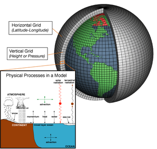
A general circulation model (GCM) is a type of climate model. It employs a mathematical model of the general circulation of a planetary atmosphere or ocean. It uses the Navier–Stokes equations on a rotating sphere with thermodynamic terms for various energy sources. These equations are the basis for computer programs used to simulate the Earth's atmosphere or oceans. Atmospheric and oceanic GCMs are key components along with sea ice and land-surface components.

In geometry, a truncated icosidodecahedron, rhombitruncated icosidodecahedron, great rhombicosidodecahedron, omnitruncated dodecahedron or omnitruncated icosahedron is an Archimedean solid, one of thirteen convex, isogonal, non-prismatic solids constructed by two or more types of regular polygon faces.

In geometry, the snub disphenoid, Siamese dodecahedron, triangular dodecahedron, trigonal dodecahedron, or dodecadeltahedron is a convex polyhedron with twelve equilateral triangles as its faces. It is not a regular polyhedron because some vertices have four faces and others have five. It is a dodecahedron, one of the eight deltahedra, and is the 84th Johnson solid. It can be thought of as a square antiprism where both squares are replaced with two equilateral triangles.
In geometry, the chamfered dodecahedron is a convex polyhedron with 80 vertices, 120 edges, and 42 faces: 30 hexagons and 12 pentagons. It is constructed as a chamfer (edge-truncation) of a regular dodecahedron. The pentagons are reduced in size and new hexagonal faces are added in place of all the original edges. Its dual is the pentakis icosidodecahedron.
GME was an operational global numerical weather prediction model run by Deutscher Wetterdienst, the German national meteorological service. The model was run using an almost uniform icosahedral-hexagonal grid. The GME grid point approach avoided the disadvantages of spectral techniques as well as the pole problem in latitude–longitude grids and provides a data structure well suited to high efficiency on distributed memory parallel computers. The GME replaced two previous models, and was first run on 1 December 1999.

Dr. André Robert was a Canadian meteorologist who pioneered the modelling the Earth's atmospheric circulation.
The Alexandrov uniqueness theorem is a rigidity theorem in mathematics, describing three-dimensional convex polyhedra in terms of the distances between points on their surfaces. It implies that convex polyhedra with distinct shapes from each other also have distinct metric spaces of surface distances, and it characterizes the metric spaces that come from the surface distances on polyhedra. It is named after Soviet mathematician Aleksandr Danilovich Aleksandrov, who published it in the 1940s.

The history of numerical weather prediction considers how current weather conditions as input into mathematical models of the atmosphere and oceans to predict the weather and future sea state has changed over the years. Though first attempted manually in the 1920s, it was not until the advent of the computer and computer simulation that computation time was reduced to less than the forecast period itself. ENIAC was used to create the first forecasts via computer in 1950, and over the years more powerful computers have been used to increase the size of initial datasets and use more complicated versions of the equations of motion. The development of global forecasting models led to the first climate models. The development of limited area (regional) models facilitated advances in forecasting the tracks of tropical cyclone as well as air quality in the 1970s and 1980s.

In mathematics, and more specifically in polyhedral combinatorics, a Goldberg polyhedron is a convex polyhedron made from hexagons and pentagons. They were first described in 1937 by Michael Goldberg (1902–1990). They are defined by three properties: each face is either a pentagon or hexagon, exactly three faces meet at each vertex, and they have rotational icosahedral symmetry. They are not necessarily mirror-symmetric; e.g. GP(5,3) and GP(3,5) are enantiomorphs of each other. A Goldberg polyhedron is a dual polyhedron of a geodesic sphere.
The Flow-following, finite-volume Icosahedral Model (FIM) is an experimental numerical weather prediction model that was developed at the Earth System Research Laboratory in the United States from 2008 to 2016.

A discrete global grid (DGG) is a mosaic that covers the entire Earth's surface. Mathematically it is a space partitioning: it consists of a set of non-empty regions that form a partition of the Earth's surface. In a usual grid-modeling strategy, to simplify position calculations, each region is represented by a point, abstracting the grid as a set of region-points. Each region or region-point in the grid is called a cell.

A geodesic polyhedron is a convex polyhedron made from triangles. They usually have icosahedral symmetry, such that they have 6 triangles at a vertex, except 12 vertices which have 5 triangles. They are the dual of corresponding Goldberg polyhedra with mostly hexagonal faces.
The order-5 truncated pentagonal hexecontahedron is a convex polyhedron with 72 faces: 60 hexagons and 12 pentagons triangular, with 210 edges, and 140 vertices. Its dual is the pentakis snub dodecahedron.

In geology, numerical modeling is a widely applied technique to tackle complex geological problems by computational simulation of geological scenarios.

The Goldberg–Coxeter construction or Goldberg–Coxeter operation is a graph operation defined on regular polyhedral graphs with degree 3 or 4. It also applies to the dual graph of these graphs, i.e. graphs with triangular or quadrilateral "faces". The GC construction can be thought of as subdividing the faces of a polyhedron with a lattice of triangular, square, or hexagonal polygons, possibly skewed with regards to the original face: it is an extension of concepts introduced by the Goldberg polyhedra and geodesic polyhedra. The GC construction is primarily studied in organic chemistry for its application to fullerenes, but it has been applied to nanoparticles, computer-aided design, basket weaving, and the general study of graph theory and polyhedra.

Snyder equal-area projection is a polyhedral map projection used in the ISEA discrete global grids. It is named for John P. Snyder, who developed the projection in the 1990s.

A polyhedral map projection is a map projection based on a spherical polyhedron. Typically, the polyhedron is overlaid on the globe, and each face of the polyhedron is transformed to a polygon or other shape in the plane. The best-known polyhedral map projection is Buckminster Fuller's Dymaxion map. When the spherical polyhedron faces are transformed to the faces of an ordinary polyhedron instead of laid flat in a plane, the result is a polyhedral globe.
{{cite conference}}: CS1 maint: numeric names: authors list (link)