This article is missing information about the case of multivariate functions and vector valued functions, which must be considered, as this article is linked to from Jacobian matrix. Please expand the article to include this information. Further details may exist on the talk page.(February 2020)
Graph of the linear function:
In calculus and related areas of mathematics, a linear function from the real numbers to the real numbers is a function whose graph (in Cartesian coordinates) is a non-vertical line in the plane.[1] The characteristic property of linear functions is that when the input variable is changed, the change in the output is proportional to the change in the input.
Such a function is called linear because its graph, the set of all points in the Cartesian plane, is a line. The coefficient a is called the slope of the function and of the line (see below).
If the slope is , this is a constant function defining a horizontal line, which some authors exclude from the class of linear functions.[3] With this definition, the degree of a linear polynomial would be exactly one, and its graph would be a line that is neither vertical nor horizontal. However, in this article, is required, so constant functions will be considered linear.
If then the linear function is said to be homogeneous. Such function defines a line that passes through the origin of the coordinate system, that is, the point . In advanced mathematics texts, the term linear function often denotes specifically homogeneous linear functions, while the term affine function is used for the general case, which includes .
The natural domain of a linear function , the set of allowed input values for x, is the entire set of real numbers, One can also consider such functions with x in an arbitrary field, taking the coefficients a, b in that field.
The graph is a non-vertical line having exactly one intersection with the y-axis, its y-intercept point The y-intercept value is also called the initial value of If the graph is a non-horizontal line having exactly one intersection with the x-axis, the x-intercept point The x-intercept value the solution of the equation is also called the root or zero of
Slope
The slope of a line is the ratio between a change in x, denoted , and the corresponding change in y, denoted
The slope of a nonvertical line is a number that measures how steeply the line is slanted (rise-over-run). If the line is the graph of the linear function , this slope is given by the constant a.
The slope measures the constant rate of change of per unit change in x: whenever the input x is increased by one unit, the output changes by a units: , and more generally for any number . If the slope is positive, , then the function is increasing; if , then is decreasing
In calculus, the derivative of a general function measures its rate of change. A linear function has a constant rate of change equal to its slope a, so its derivative is the constant function .
The fundamental idea of differential calculus is that any smooth function (not necessarily linear) can be closely approximated near a given point by a unique linear function. The derivative is the slope of this linear function, and the approximation is: for . The graph of the linear approximation is the tangent line of the graph at the point . The derivative slope generally varies with the point c. Linear functions can be characterized as the only real functions whose derivative is constant: if for all x, then for .
Slope-intercept, point-slope, and two-point forms
A given linear function can be written in several standard formulas displaying its various properties. The simplest is the slope-intercept form:
,
from which one can immediately see the slope a and the initial value , which is the y-intercept of the graph .
Given a slope a and one known value , we write the point-slope form:
.
In graphical terms, this gives the line with slope a passing through the point .
The two-point form starts with two known values and . One computes the slope and inserts this into the point-slope form:
.
Its graph is the unique line passing through the points . The equation may also be written to emphasize the constant slope:
.
Relationship with linear equations
Linear functions commonly arise from practical problems involving variables with a linear relationship, that is, obeying a linear equation. If , one can solve this equation for y, obtaining
where we denote and . That is, one may consider y as a dependent variable (output) obtained from the independent variable (input) x via a linear function: . In the xy-coordinate plane, the possible values of form a line, the graph of the function . If in the original equation, the resulting line is vertical, and cannot be written as .
The features of the graph can be interpreted in terms of the variables x and y. The y-intercept is the initial value at . The slope a measures the rate of change of the output y per unit change in the input x. In the graph, moving one unit to the right (increasing x by 1) moves the y-value up by a: that is, . Negative slope a indicates a decrease in y for each increase in x.
For example, the linear function has slope , y-intercept point , and x-intercept point .
Example
Suppose salami and sausage cost €6 and €3 per kilogram, and we wish to buy €12 worth. How much of each can we purchase? If x kilograms of salami and y kilograms of sausage costs a total of €12 then, €6×x + €3×y = €12. Solving for y gives the point-slope form , as above. That is, if we first choose the amount of salami x, the amount of sausage can be computed as a function . Since salami costs twice as much as sausage, adding one kilo of salami decreases the sausage by 2 kilos: , and the slope is −2. The y-intercept point corresponds to buying only 4kg of sausage; while the x-intercept point corresponds to buying only 2kg of salami.
Note that the graph includes points with negative values of x or y, which have no meaning in terms of the original variables (unless we imagine selling meat to the butcher). Thus we should restrict our function to the domain .
Also, we could choose y as the independent variable, and compute x by the inverse linear function: over the domain .
Relationship with other classes of functions
If the coefficient of the variable is not zero (a ≠ 0), then a linear function is represented by a degree 1 polynomial (also called a linear polynomial), otherwise it is a constant function – also a polynomial function, but of zero degree.
A straight line, when drawn in a different kind of coordinate system may represent other functions.
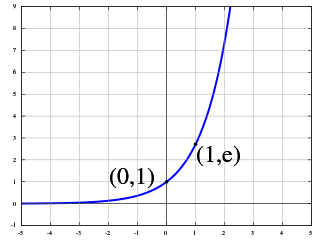
For example, it may represent an exponential function when its values are expressed in the logarithmic scale. It means that when log(g(x)) is a linear function of x, the function g is exponential. With linear functions, increasing the input by one unit causes the output to increase by a fixed amount, which is the slope of the graph of the function. With exponential functions, increasing the input by one unit causes the output to increase by a fixed multiple, which is known as the base of the exponential function.
If botharguments and values of a function are in the logarithmic scale (i.e., when log(y) is a linear function of log(x)), then the straight line represents a power law:
Archimedean spiral defined by the polar equation r = 1⁄2θ + 2
On the other hand, the graph of a linear function in terms of polar coordinates:
In analytic geometry, an asymptote of a curve is a line such that the distance between the curve and the line approaches zero as one or both of the x or y coordinates tends to infinity. In projective geometry and related contexts, an asymptote of a curve is a line which is tangent to the curve at a point at infinity.
In mathematics, an equation is a mathematical formula that expresses the equality of two expressions, by connecting them with the equals sign =. The word equation and its cognates in other languages may have subtly different meanings; for example, in French an équation is defined as containing one or more variables, while in English, any well-formed formula consisting of two expressions related with an equals sign is an equation.
The exponential function is a mathematical function denoted by or . Unless otherwise specified, the term generally refers to the positive-valued function of a real variable, although it can be extended to the complex numbers or generalized to other mathematical objects like matrices or Lie algebras. The exponential function originated from the operation of taking powers of a number, but various modern definitions allow it to be rigorously extended to all real arguments , including irrational numbers. Its ubiquitous occurrence in pure and applied mathematics led mathematician Walter Rudin to consider the exponential function to be "the most important function in mathematics".
In mathematics, a linear equation is an equation that may be put in the form where are the variables, and are the coefficients, which are often real numbers. The coefficients may be considered as parameters of the equation and may be arbitrary expressions, provided they do not contain any of the variables. To yield a meaningful equation, the coefficients are required to not all be zero.
In mathematics, a polynomial is a mathematical expression consisting of indeterminates and coefficients, that involves only the operations of addition, subtraction, multiplication, and positive-integer powers of variables. An example of a polynomial of a single indeterminate x is x2 − 4x + 7. An example with three indeterminates is x3 + 2xyz2 − yz + 1.
Quadratic programming (QP) is the process of solving certain mathematical optimization problems involving quadratic functions. Specifically, one seeks to optimize a multivariate quadratic function subject to linear constraints on the variables. Quadratic programming is a type of nonlinear programming.
In mathematics, differential calculus is a subfield of calculus that studies the rates at which quantities change. It is one of the two traditional divisions of calculus, the other being integral calculus—the study of the area beneath a curve.
In mathematics, the term linear is used in two distinct senses for two different properties:
In mathematics, the term linear function refers to two distinct but related notions:
In mathematics, a quadratic polynomial is a polynomial of degree two in one or more variables. A quadratic function is the polynomial function defined by a quadratic polynomial. Before the 20th century, the distinction was unclear between a polynomial and its associated polynomial function; so "quadratic polynomial" and "quadratic function" were almost synonymous. This is still the case in many elementary courses, where both terms are often abbreviated as "quadratic".
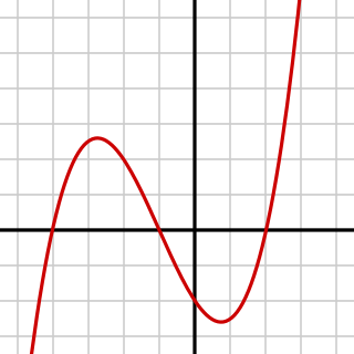
In mathematics, a cubic function is a function of the form that is, a polynomial function of degree three. In many texts, the coefficientsa, b, c, and d are supposed to be real numbers, and the function is considered as a real function that maps real numbers to real numbers or as a complex function that maps complex numbers to complex numbers. In other cases, the coefficients may be complex numbers, and the function is a complex function that has the set of the complex numbers as its codomain, even when the domain is restricted to the real numbers.
In mathematics, a real-valued function is called convex if the line segment between any two distinct points on the graph of the function lies above the graph between the two points. Equivalently, a function is convex if its epigraph is a convex set. In simple terms, a convex function graph is shaped like a cup , while a concave function's graph is shaped like a cap .
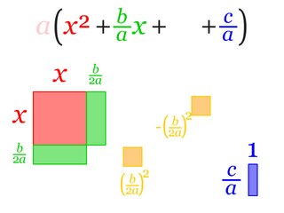
In elementary algebra, completing the square is a technique for converting a quadratic polynomial of the form
In mathematics, a constant function is a function whose (output) value is the same for every input value. For example, the function y(x) = 4 is a constant function because the value of y(x) is 4 regardless of the input value x (see image).
In mathematics, a rational function is any function that can be defined by a rational fraction, which is an algebraic fraction such that both the numerator and the denominator are polynomials. The coefficients of the polynomials need not be rational numbers; they may be taken in any field K. In this case, one speaks of a rational function and a rational fraction over K. The values of the variables may be taken in any field L containing K. Then the domain of the function is the set of the values of the variables for which the denominator is not zero, and the codomain is L.
In science and engineering, a log–log graph or log–log plot is a two-dimensional graph of numerical data that uses logarithmic scales on both the horizontal and vertical axes. Power functions – relationships of the form – appear as straight lines in a log–log graph, with the exponent corresponding to the slope, and the coefficient corresponding to the intercept. Thus these graphs are very useful for recognizing these relationships and estimating parameters. Any base can be used for the logarithm, though most commonly base 10 are used.
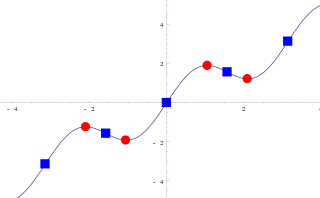
In mathematics, a critical point is the argument of a function where the function derivative is zero . The value of the function at a critical point is a critical value.
In mathematics, a variable is a symbol that represents a mathematical object. A variable may represent a number, a vector, a matrix, a function, the argument of a function, a set, or an element of a set.
In science and engineering, a semi-log plot/graph or semi-logarithmicplot/graph has one axis on a logarithmic scale, the other on a linear scale. It is useful for data with exponential relationships, where one variable covers a large range of values, or to zoom in and visualize that - what seems to be a straight line in the beginning - is in fact the slow start of a logarithmic curve that is about to spike and changes are much bigger than thought initially.
Most of the terms listed in Wikipedia glossaries are already defined and explained within Wikipedia itself. However, glossaries like this one are useful for looking up, comparing and reviewing large numbers of terms together. You can help enhance this page by adding new terms or writing definitions for existing ones.
References
James Stewart (2012), Calculus: Early Transcendentals, edition 7E, Brooks/Cole. ISBN978-0-538-49790-9
This page is based on this Wikipedia article Text is available under the CC BY-SA 4.0 license; additional terms may apply. Images, videos and audio are available under their respective licenses.