Exponential growth is a process that increases quantity over time at an ever-increasing rate. It occurs when the instantaneous rate of change (that is, the derivative) of a quantity with respect to time is proportional to the quantity itself. Described as a function, a quantity undergoing exponential growth is an exponential function of time, that is, the variable representing time is the exponent (in contrast to other types of growth, such as quadratic growth). Exponential growth is the inverse of logarithmic growth.
If the constant of proportionality is negative, then the quantity decreases over time, and is said to be undergoing exponential decay instead. In the case of a discrete domain of definition with equal intervals, it is also called geometric growth or geometric decay since the function values form a geometric progression.
The formula for exponential growth of a variable x at the growth rate r, as time t goes on in discrete intervals (that is, at integer times0,1,2,3,...), is
where x0 is the value of x at time 0. The growth of a bacterial colony is often used to illustrate it. One bacterium splits itself into two, each of which splits itself resulting in four, then eight, 16, 32, and so on. The amount of increase keeps increasing because it is proportional to the ever-increasing number of bacteria. Growth like this is observed in real-life activity or phenomena, such as the spread of virus infection, the growth of debt due to compound interest, and the spread of viral videos. In real cases, initial exponential growth often does not last forever, instead slowing down eventually due to upper limits caused by external factors and turning into logistic growth.
Terms like "exponential growth" are sometimes incorrectly interpreted as "rapid growth". Indeed, something that grows exponentially can in fact be growing slowly at first.[1][2]
Examples
Bacteria exhibit exponential growth under optimal conditions.
The number of microorganisms in a culture will increase exponentially until an essential nutrient is exhausted, so there is no more of that nutrient for more organisms to grow. Typically the first organism splits into two daughter organisms, who then each split to form four, who split to form eight, and so on. Because exponential growth indicates constant growth rate, it is frequently assumed that exponentially growing cells are at a steady-state. However, cells can grow exponentially at a constant rate while remodeling their metabolism and gene expression.[3]
A virus (for example COVID-19, or smallpox) typically will spread exponentially at first, if no artificial immunization is available. Each infected person can infect multiple new people.
Physics
Avalanche breakdown within a dielectric material. A free electron becomes sufficiently accelerated by an externally applied electrical field that it frees up additional electrons as it collides with atoms or molecules of the dielectric media. These secondary electrons also are accelerated, creating larger numbers of free electrons. The resulting exponential growth of electrons and ions may rapidly lead to complete dielectric breakdown of the material.
Nuclear chain reaction (the concept behind nuclear reactors and nuclear weapons). Each uraniumnucleus that undergoes fission produces multiple neutrons, each of which can be absorbed by adjacent uranium atoms, causing them to fission in turn. If the probability of neutron absorption exceeds the probability of neutron escape (a function of the shape and mass of the uranium), the production rate of neutrons and induced uranium fissions increases exponentially, in an uncontrolled reaction. "Due to the exponential rate of increase, at any point in the chain reaction 99% of the energy will have been released in the last 4.6 generations. It is a reasonable approximation to think of the first 53 generations as a latency period leading up to the actual explosion, which only takes 3–4 generations."[4]
Positive feedback within the linear range of electrical or electroacoustic amplification can result in the exponential growth of the amplified signal, although resonance effects may favor some component frequencies of the signal over others.
Economics
Economic growth is expressed in percentage terms, implying exponential growth.
Pyramid schemes or Ponzi schemes also show this type of growth resulting in high profits for a few initial investors and losses among great numbers of investors.
Computer science
Processing power of computers. See also Moore's law and technological singularity. (Under exponential growth, there are no singularities. The singularity here is a metaphor, meant to convey an unimaginable future. The link of this hypothetical concept with exponential growth is most vocally made by futurist Ray Kurzweil.)
In computational complexity theory, computer algorithms of exponential complexity require an exponentially increasing amount of resources (e.g. time, computer memory) for only a constant increase in problem size. So for an algorithm of time complexity 2x, if a problem of size x = 10 requires 10 seconds to complete, and a problem of size x = 11 requires 20 seconds, then a problem of size x = 12 will require 40 seconds. This kind of algorithm typically becomes unusable at very small problem sizes, often between 30 and 100 items (most computer algorithms need to be able to solve much larger problems, up to tens of thousands or even millions of items in reasonable times, something that would be physically impossible with an exponential algorithm). Also, the effects of Moore's Law do not help the situation much because doubling processor speed merely increases the feasible problem size by a constant. E.g. if a slow processor can solve problems of size x in time t, then a processor twice as fast could only solve problems of size x + constant in the same time t. So exponentially complex algorithms are most often impractical, and the search for more efficient algorithms is one of the central goals of computer science today.
Internet phenomena
Internet contents, such as internet memes or videos, can spread in an exponential manner, often said to "go viral" as an analogy to the spread of viruses.[6] With media such as social networks, one person can forward the same content to many people simultaneously, who then spread it to even more people, and so on, causing rapid spread.[7] For example, the video Gangnam Style was uploaded to YouTube on 15 July 2012, reaching hundreds of thousands of viewers on the first day, millions on the twentieth day, and was cumulatively viewed by hundreds of millions in less than two months.[6][8]
Basic formula
exponential growth: exponential growth:
A quantity x depends exponentially on time t if
where the constant a is the initial value of x,
the constant b is a positive growth factor, and τ is the time constant—the time required for x to increase by one factor of b:
If τ > 0 and b > 1, then x has exponential growth. If τ < 0 and b > 1, or τ > 0 and 0 < b < 1, then x has exponential decay.
Example: If a species of bacteria doubles every ten minutes, starting out with only one bacterium, how many bacteria would be present after one hour? The question implies a = 1, b = 2 and τ = 10 min.
After one hour, or six ten-minute intervals, there would be sixty-four bacteria.
Many pairs (b, τ) of a dimensionless non-negative number b and an amount of time τ (a physical quantity which can be expressed as the product of a number of units and a unit of time) represent the same growth rate, with τ proportional to log b. For any fixed b not equal to 1 (e.g. e or 2), the growth rate is given by the non-zero time τ. For any non-zero time τ the growth rate is given by the dimensionless positive numberb.
Thus the law of exponential growth can be written in different but mathematically equivalent forms, by using a different base. The most common forms are the following:
where x0 expresses the initial quantity x(0).
Parameters (negative in the case of exponential decay):
The percent increase r (a dimensionless number) in a period p.
The quantities k, τ, and T, and for a given p also r, have a one-to-one connection given by the following equation (which can be derived by taking the natural logarithm of the above):
where k = 0 corresponds to r = 0 and to τ and T being infinite.
If p is the unit of time the quotient t/p is simply the number of units of time. Using the notation t for the (dimensionless) number of units of time rather than the time itself, t/p can be replaced by t, but for uniformity this has been avoided here. In this case the division by p in the last formula is not a numerical division either, but converts a dimensionless number to the correct quantity including unit.
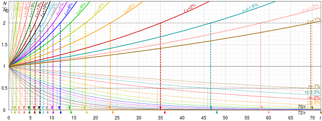
A popular approximated method for calculating the doubling time from the growth rate is the rule of 70, that is, .
Graphs comparing doubling times and half lives of exponential growths (bold lines) and decay (faint lines), and their 70/t and 72/t approximations. In the SVG version, hover over a graph to highlight it and its complement.
Reformulation as log-linear growth
If a variable x exhibits exponential growth according to , then the log (to any base) of xgrows linearly over time, as can be seen by taking logarithms of both sides of the exponential growth equation:
This allows an exponentially growing variable to be modeled with a log-linear model. For example, if one wishes to empirically estimate the growth rate from intertemporal data on x, one can linearly regresslog x on t.
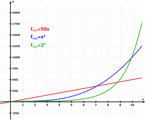
In the long run, exponential growth of any kind will overtake linear growth of any kind (that is the basis of the Malthusian catastrophe) as well as any polynomial growth, that is, for all α:
Growth rates may also be faster than exponential. In the most extreme case, when growth increases without bound in finite time, it is called hyperbolic growth. In between exponential and hyperbolic growth lie more classes of growth behavior, like the hyperoperations beginning at tetration, and , the diagonal of the Ackermann function.
Logistic growth
The J-shaped exponential growth (left, blue) and the S-shaped logistic growth (right, red).
In reality, initial exponential growth is often not sustained forever. After some period, it will be slowed by external or environmental factors. For example, population growth may reach an upper limit due to resource limitations.[9] In 1845, the Belgian mathematician Pierre François Verhulst first proposed a mathematical model of growth like this, called the "logistic growth".[10]
Limitations of models
Exponential growth models of physical phenomena only apply within limited regions, as unbounded growth is not physically realistic. Although growth may initially be exponential, the modelled phenomena will eventually enter a region in which previously ignored negative feedback factors become significant (leading to a logistic growth model) or other underlying assumptions of the exponential growth model, such as continuity or instantaneous feedback, break down.
Studies show that human beings have difficulty understanding exponential growth. Exponential growth bias is the tendency to underestimate compound growth processes. This bias can have financial implications as well.[11]
According to an old legend, vizier Sissa Ben Dahir presented an Indian King Sharim with a beautiful handmade chessboard. The king asked what he would like in return for his gift and the courtier surprised the king by asking for one grain of rice on the first square, two grains on the second, four grains on the third, etc. The king readily agreed and asked for the rice to be brought. All went well at first, but the requirement for 2n−1 grains on the nth square demanded over a million grains on the 21st square, more than a million million (a.k.a. trillion) on the 41st and there simply was not enough rice in the whole world for the final squares. (From Swirski, 2006)[12]
The second half of the chessboard is the time when an exponentially growing influence is having a significant economic impact on an organization's overall business strategy.
Water lily
French children are offered a riddle, which appears to be an aspect of exponential growth: "the apparent suddenness with which an exponentially growing quantity approaches a fixed limit". The riddle imagines a water lily plant growing in a pond. The plant doubles in size every day and, if left alone, it would smother the pond in 30 days killing all the other living things in the water. Day after day, the plant's growth is small, so it is decided that it won't be a concern until it covers half of the pond. Which day will that be? The 29th day, leaving only one day to save the pond.[13][12]
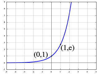
The number e is a mathematical constant approximately equal to 2.71828 that can be characterized in many ways. It is the base of the natural logarithm function. It is the limit of as n tends to infinity, an expression that arises in the computation of compound interest. It is the value at 1 of the (natural) exponential function, commonly denoted It is also the sum of the infinite series
The exponential function is a mathematical function denoted by or . Unless otherwise specified, the term generally refers to the positive-valued function of a real variable, although it can be extended to the complex numbers or generalized to other mathematical objects like matrices or Lie algebras. The exponential function originated from the operation of taking powers of a number, but various modern definitions allow it to be rigorously extended to all real arguments , including irrational numbers. Its ubiquitous occurrence in pure and applied mathematics led mathematician Walter Rudin to consider the exponential function to be "the most important function in mathematics".
Half-life is the time required for a quantity to reduce to half of its initial value. The term is commonly used in nuclear physics to describe how quickly unstable atoms undergo radioactive decay or how long stable atoms survive. The term is also used more generally to characterize any type of exponential decay. For example, the medical sciences refer to the biological half-life of drugs and other chemicals in the human body. The converse of half-life is doubling time.
In statistics, a normal distribution or Gaussian distribution is a type of continuous probability distribution for a real-valued random variable. The general form of its probability density function is
A chirp is a signal in which the frequency increases (up-chirp) or decreases (down-chirp) with time. In some sources, the term chirp is used interchangeably with sweep signal. It is commonly applied to sonar, radar, and laser systems, and to other applications, such as in spread-spectrum communications. This signal type is biologically inspired and occurs as a phenomenon due to dispersion. It is usually compensated for by using a matched filter, which can be part of the propagation channel. Depending on the specific performance measure, however, there are better techniques both for radar and communication. Since it was used in radar and space, it has been adopted also for communication standards. For automotive radar applications, it is usually called linear frequency modulated waveform (LFMW).
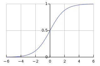
A logistic function or logistic curve is a common S-shaped curve with the equation
In mathematics, Stirling's approximation is an asymptotic approximation for factorials. It is a good approximation, leading to accurate results even for small values of . It is named after James Stirling, though a related but less precise result was first stated by Abraham de Moivre.
In applied mathematics, discretization is the process of transferring continuous functions, models, variables, and equations into discrete counterparts. This process is usually carried out as a first step toward making them suitable for numerical evaluation and implementation on digital computers. Dichotomization is the special case of discretization in which the number of discrete classes is 2, which can approximate a continuous variable as a binary variable.
A quantity is subject to exponential decay if it decreases at a rate proportional to its current value. Symbolically, this process can be expressed by the following differential equation, where N is the quantity and λ (lambda) is a positive rate called the exponential decay constant, disintegration constant, rate constant, or transformation constant:
The step response of a system in a given initial state consists of the time evolution of its outputs when its control inputs are Heaviside step functions. In electronic engineering and control theory, step response is the time behaviour of the outputs of a general system when its inputs change from zero to one in a very short time. The concept can be extended to the abstract mathematical notion of a dynamical system using an evolution parameter.
In statistics, a generalized linear model (GLM) is a flexible generalization of ordinary linear regression. The GLM generalizes linear regression by allowing the linear model to be related to the response variable via a link function and by allowing the magnitude of the variance of each measurement to be a function of its predicted value.
The equilibrium constant of a chemical reaction is the value of its reaction quotient at chemical equilibrium, a state approached by a dynamic chemical system after sufficient time has elapsed at which its composition has no measurable tendency towards further change. For a given set of reaction conditions, the equilibrium constant is independent of the initial analytical concentrations of the reactant and product species in the mixture. Thus, given the initial composition of a system, known equilibrium constant values can be used to determine the composition of the system at equilibrium. However, reaction parameters like temperature, solvent, and ionic strength may all influence the value of the equilibrium constant.
In system analysis, among other fields of study, a linear time-invariant (LTI) system is a system that produces an output signal from any input signal subject to the constraints of linearity and time-invariance; these terms are briefly defined below. These properties apply (exactly or approximately) to many important physical systems, in which case the response y(t) of the system to an arbitrary input x(t) can be found directly using convolution: y(t) = (x ∗ h)(t) where h(t) is called the system's impulse response and ∗ represents convolution (not to be confused with multiplication). What's more, there are systematic methods for solving any such system (determining h(t)), whereas systems not meeting both properties are generally more difficult (or impossible) to solve analytically. A good example of an LTI system is any electrical circuit consisting of resistors, capacitors, inductors and linear amplifiers.
Nondimensionalization is the partial or full removal of physical dimensions from an equation involving physical quantities by a suitable substitution of variables. This technique can simplify and parameterize problems where measured units are involved. It is closely related to dimensional analysis. In some physical systems, the term scaling is used interchangeably with nondimensionalization, in order to suggest that certain quantities are better measured relative to some appropriate unit. These units refer to quantities intrinsic to the system, rather than units such as SI units. Nondimensionalization is not the same as converting extensive quantities in an equation to intensive quantities, since the latter procedure results in variables that still carry units.
In mathematics, in the area of complex analysis, Nachbin's theorem is commonly used to establish a bound on the growth rates for an analytic function. This article provides a brief review of growth rates, including the idea of a function of exponential type. Classification of growth rates based on type help provide a finer tool than big O or Landau notation, since a number of theorems about the analytic structure of the bounded function and its integral transforms can be stated. In particular, Nachbin's theorem may be used to give the domain of convergence of the generalized Borel transform, given below.
In complex analysis, a branch of mathematics, a holomorphic function is said to be of exponential type C if its growth is bounded by the exponential function for some real-valued constant as . When a function is bounded in this way, it is then possible to express it as certain kinds of convergent summations over a series of other complex functions, as well as understanding when it is possible to apply techniques such as Borel summation, or, for example, to apply the Mellin transform, or to perform approximations using the Euler–Maclaurin formula. The general case is handled by Nachbin's theorem, which defines the analogous notion of -type for a general function as opposed to .
In probability theory, the Gillespie algorithm generates a statistically correct trajectory of a stochastic equation system for which the reaction rates are known. It was created by Joseph L. Doob and others, presented by Dan Gillespie in 1976, and popularized in 1977 in a paper where he uses it to simulate chemical or biochemical systems of reactions efficiently and accurately using limited computational power. As computers have become faster, the algorithm has been used to simulate increasingly complex systems. The algorithm is particularly useful for simulating reactions within cells, where the number of reagents is low and keeping track of every single reaction is computationally feasible. Mathematically, it is a variant of a dynamic Monte Carlo method and similar to the kinetic Monte Carlo methods. It is used heavily in computational systems biology.
In theory of vibrations, Duhamel's integral is a way of calculating the response of linear systems and structures to arbitrary time-varying external perturbation.
In statistics, the Kendall rank correlation coefficient, commonly referred to as Kendall's τ coefficient, is a statistic used to measure the ordinal association between two measured quantities. A τ test is a non-parametric hypothesis test for statistical dependence based on the τ coefficient. It is a measure of rank correlation: the similarity of the orderings of the data when ranked by each of the quantities. It is named after Maurice Kendall, who developed it in 1938, though Gustav Fechner had proposed a similar measure in the context of time series in 1897.
A double exponential function is a constant raised to the power of an exponential function. The general formula is (where a>1 and b>1), which grows much more quickly than an exponential function. For example, if a = b = 10:
↑ Stango, Victor; Zinman, Jonathan (2009). "Exponential Growth Bias and Household Finance". The Journal of Finance. 64 (6): 2807–2849. doi:10.1111/j.1540-6261.2009.01518.x.
1 2 Porritt, Jonathan (2005). Capitalism: as if the world matters. London: Earthscan. p.49. ISBN1-84407-192-8.
↑ Meadows, Donella (2004). The Limits to Growth: The 30-Year Update. Chelsea Green Publishing. p.21. ISBN9781603581554.
Meadows, Donella H., Dennis L. Meadows, Jørgen Randers, and William W. Behrens III. (1972) The Limits to Growth. New York: University Books. ISBN0-87663-165-0
Porritt, J. Capitalism as if the world matters, Earthscan 2005. ISBN1-84407-192-8
Swirski, Peter. Of Literature and Knowledge: Explorations in Narrative Thought Experiments, Evolution, and Game Theory. New York: Routledge. ISBN0-415-42060-1
Thomson, David G. Blueprint to a Billion: 7 Essentials to Achieve Exponential Growth, Wiley Dec 2005, ISBN0-471-74747-5
This page is based on this Wikipedia article Text is available under the CC BY-SA 4.0 license; additional terms may apply. Images, videos and audio are available under their respective licenses.


