Non-uniform rational B-spline

A NURBS curve. (See also: the animated creation of a NURBS spline.)

A NURBS surface

Non-uniform rational basis spline (NURBS) is a mathematical model using basis splines (B-splines) that is commonly used in computer graphics for representing curves and surfaces. It offers great flexibility and precision for handling both analytic (defined by common mathematical formulae) and modeled shapes. It is a type of curve modeling, as opposed to polygonal modeling or digital sculpting. NURBS curves are commonly used in computer-aided design (CAD), manufacturing (CAM), and engineering (CAE). They are part of numerous industry-wide standards, such as IGES, STEP, ACIS, and PHIGS. Tools for creating and editing NURBS surfaces are found in various 3D graphics, rendering, ^[1] and animation software packages.

They can be efficiently handled by computer programs yet allow for easy human interaction. NURBS surfaces are functions of two parameters mapping to a surface in three-dimensional space. The shape of the surface is determined by control points. In a compact form, NURBS surfaces can represent simple geometrical shapes. For complex organic shapes, T-splines and subdivision surfaces are more suitable because they halve the number of control points in comparison with the NURBS surfaces.

In general, editing NURBS curves and surfaces is intuitive and predictable.^{[ citation needed ]} Control points are always either connected directly to the curve or surface, or else act as if they were connected by a rubber band. Depending on the type of user interface, the editing of NURBS curves and surfaces can be via their control points (similar to Bézier curves) or via higher level tools such as spline modeling and hierarchical editing.

History

A flat spline, a physical manifestation of the spline as a mathematical concept

Before computers, designs were drawn by hand on paper with various drafting tools. Rulers were used for straight lines, compasses for circles, and protractors for angles. But many shapes, such as the freeform curve of a ship's bow, could not be drawn with these tools. Although such curves could be drawn freehand at the drafting board, shipbuilders often needed a life-size version which could not be done by hand. Such large drawings were done with the help of flexible strips of wood, called splines. The splines were held in place at a number of predetermined points, called "ducks" (which were made of lead and about 3 inches long: the "beak" of the "duck" pushed against the spline; the old yacht-design books assumed these methods); between the ducks, the elasticity of the spline material caused the strip to take the shape that minimized the energy of bending, thus creating the smoothest possible shape that fit the constraints. The shape could be adjusted by moving the ducks. ^{[2] [3]}

In 1946, mathematicians started studying the spline shape, and derived the piecewise polynomial formula known as the spline curve or spline function. I. J. Schoenberg gave the spline function its name after its resemblance to the mechanical spline used by draftsmen. ^[4]

As computers were introduced into the design process, the physical properties of such splines were investigated so that they could be modelled with mathematical precision and reproduced where needed. Pioneering work was done in France by Renault engineer Pierre Bézier, and Citroën's physicist and mathematician Paul de Casteljau. They worked nearly parallel to each other, but because Bézier published the results of his work, Bézier curves were named after him, while de Casteljau's name is only associated with related algorithms.

NURBS were initially used only in the proprietary CAD packages of car companies. Later they became part of standard computer graphics packages.

Real-time, interactive rendering of NURBS curves and surfaces was first made commercially available on Silicon Graphics workstations in 1989. In 1993, the first interactive NURBS modeller for PCs, called NöRBS, was developed by CAS Berlin, a small startup company cooperating with the Technical University of Berlin.^{[ citation needed ]}

Continuity

Main article: Smooth function

A surface under construction, e.g. the hull of a motor yacht, is usually composed of several NURBS surfaces known as NURBS patches (or just patches). These surface patches should be fitted together in such a way that the boundaries are invisible. This is mathematically expressed by the concept of geometric continuity.

Higher-level tools exist that benefit from the ability of NURBS to create and establish geometric continuity of different levels:

• Positional continuity (G⁰) holds whenever the end positions of two curves or surfaces coincide. The curves or surfaces may still meet at an angle, giving rise to a sharp corner or edge and causing broken highlights.
• Tangential continuity (G¹) requires the end vectors of the curves or surfaces to be parallel and pointing the same way, ruling out sharp edges. Because highlights falling on a tangentially continuous edge are always continuous and thus look natural, this level of continuity can often be sufficient.
• Curvature continuity (G²) further requires the end vectors to be of the same length and rate of length change. Highlights falling on a curvature-continuous edge do not display any change, causing the two surfaces to appear as one. This can be visually recognized as "perfectly smooth". This level of continuity is very useful in the creation of models that require many bi-cubic patches composing one continuous surface.

Geometric continuity mainly refers to the shape of the resulting surface; since NURBS surfaces are functions, it is also possible to discuss the derivatives of the surface with respect to the parameters. This is known as parametric continuity. Parametric continuity of a given degree implies geometric continuity of that degree.

First- and second-level parametric continuity (C⁰ and C¹) are for practical purposes identical to positional and tangential (G⁰ and G¹) continuity. Third-level parametric continuity (C²), however, differs from curvature continuity in that its parameterization is also continuous. In practice, C² continuity is easier to achieve if uniform B-splines are used.

The definition of Cⁿ continuity requires that the nth derivative of adjacent curves/surfaces (${\displaystyle d^{n}C(u)/du^{n}}$) are equal at a joint. ^[5] Note that the (partial) derivatives of curves and surfaces are vectors that have a direction and a magnitude; both should be equal.

Highlights and reflections can reveal the perfect smoothing, which is otherwise practically impossible to achieve without NURBS surfaces that have at least G² continuity. This same principle is used as one of the surface evaluation methods whereby a ray-traced or reflection-mapped image of a surface with white stripes reflecting on it will show even the smallest deviations on a surface or set of surfaces. This method is derived from car prototyping wherein surface quality is inspected by checking the quality of reflections of a neon-light ceiling on the car surface. This method is also known as "Zebra analysis".

Technical specifications

A NURBS curve is defined by its order, a set of weighted control points, and a knot vector. ^[6] NURBS curves and surfaces are generalizations of both B-splines and Bézier curves and surfaces, the primary difference being the weighting of the control points, which makes NURBS curves rational.

(Non-rational, aka simple, B-splines are a special case/subset of rational B-splines, where each control point is a regular non-homogenous coordinate [no 'w'] rather than a homogeneous coordinate. ^[7] That is equivalent to having weight "1" at each control point; Rational B-splines use the 'w' of each control point as a weight. ^[8] )

By using a two-dimensional grid of control points, NURBS surfaces including planar patches and sections of spheres can be created. These are parametrized with two variables (typically called s and t or u and v). This can be extended to arbitrary dimensions to create NURBS mapping ${\displaystyle \mathbb {R} ^{n}\to \mathbb {R} ^{n}}$.

NURBS curves and surfaces are useful for a number of reasons:

• The set of NURBS for a given order is invariant under affine transformations: ^[9] operations like rotations and translations can be applied to NURBS curves and surfaces by applying them to their control points.
• They offer one common mathematical form for both standard analytical shapes (e.g., conics) and free-form shapes.
• They provide the flexibility to design a large variety of shapes.
• They reduce the memory consumption when storing shapes (compared to simpler methods).
• They can be evaluated reasonably quickly by numerically stable and accurate algorithms.

Here, NURBS is mostly discussed in one dimension (curves); it can be generalized to two (surfaces) or even more dimensions.

Order

The order of a NURBS curve defines the number of nearby control points that influence any given point on the curve. The curve is represented mathematically by a polynomial of degree one less than the order of the curve. Hence, second-order curves (which are represented by linear polynomials) are called linear curves, third-order curves are called quadratic curves, and fourth-order curves are called cubic curves. The number of control points must be greater than or equal to the order of the curve.

In practice, cubic curves are the ones most commonly used. Fifth- and sixth-order curves are sometimes useful, especially for obtaining continuous higher order derivatives, but curves of higher orders are practically never used because they lead to internal numerical problems and tend to require disproportionately large calculation times.

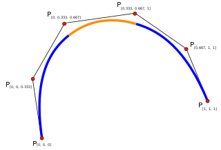
Control points

Three-dimensional NURBS surfaces can have complex, organic shapes. Control points influence the directions the surface takes. A separate square below the control cage delineates the X and Y extents of the surface.

The control points determine the shape of the curve. ^[10] Typically, each point of the curve is computed by taking a weighted sum of a number of control points. The weight of each point varies according to the governing parameter. For a curve of degree d, the weight of any control point is only nonzero in d+1 intervals of the parameter space. Within those intervals, the weight changes according to a polynomial function (basis functions) of degree d. At the boundaries of the intervals, the basis functions go smoothly to zero, the smoothness being determined by the degree of the polynomial.

As an example, the basis function of degree one is a triangle function. It rises from zero to one, then falls to zero again. While it rises, the basis function of the previous control point falls. In that way, the curve interpolates between the two points, and the resulting curve is a polygon, which is continuous, but not differentiable at the interval boundaries, or knots. Higher degree polynomials have correspondingly more continuous derivatives. Note that within the interval the polynomial nature of the basis functions and the linearity of the construction make the curve perfectly smooth, so it is only at the knots that discontinuity can arise.

In many applications the fact that a single control point only influences those intervals where it is active is a highly desirable property, known as local support. In modeling, it allows the changing of one part of a surface while keeping other parts unchanged.

Adding more control points allows better approximation to a given curve, although only a certain class of curves can be represented exactly with a finite number of control points. NURBS curves also feature a scalar weight for each control point. This allows for more control over the shape of the curve without unduly raising the number of control points. In particular, it adds conic sections like circles and ellipses to the set of curves that can be represented exactly. The term rational in NURBS refers to these weights.

The control points can have any dimensionality. One-dimensional points just define a scalar function of the parameter. These are typically used in image processing programs to tune the brightness and color curves. Three-dimensional control points are used abundantly in 3D modeling, where they are used in the everyday meaning of the word 'point', a location in 3D space. Multi-dimensional points might be used to control sets of time-driven values, e.g. the different positional and rotational settings of a robot arm. NURBS surfaces are just an application of this. Each control 'point' is actually a full vector of control points, defining a curve. These curves share their degree and the number of control points, and span one dimension of the parameter space. By interpolating these control vectors over the other dimension of the parameter space, a continuous set of curves is obtained, defining the surface.

Knot vector

The knot vector is a sequence of parameter values that determines where and how the control points affect the NURBS curve. The number of knots is always equal to the number of control points plus curve degree plus one (i.e. number of control points plus curve order). The knot vector divides the parametric space in the intervals mentioned before, usually referred to as knot spans. Each time the parameter value enters a new knot span, a new control point becomes active, while an old control point is discarded. It follows that the values in the knot vector should be in nondecreasing order, so (0, 0, 1, 2, 3, 3) is valid while (0, 0, 2, 1, 3, 3) is not.

Consecutive knots can have the same value. This then defines a knot span of zero length, which implies that two control points are activated at the same time (and of course two control points become deactivated). This has impact on continuity of the resulting curve or its higher derivatives; for instance, it allows the creation of corners in an otherwise smooth NURBS curve. A number of coinciding knots is sometimes referred to as a knot with a certain multiplicity. Knots with multiplicity two or three are known as double or triple knots. The multiplicity of a knot is limited to the degree of the curve; since a higher multiplicity would split the curve into disjoint parts and it would leave control points unused. For first-degree NURBS, each knot is paired with a control point.

The knot vector usually starts with a knot that has multiplicity equal to the order. This makes sense, since this activates the control points that have influence on the first knot span. Similarly, the knot vector usually ends with a knot of that multiplicity. Curves with such knot vectors start and end in a control point.

The values of the knots control the mapping between the input parameter and the corresponding NURBS value. For example, if a NURBS describes a path through space over time, the knots control the time that the function proceeds past the control points. For the purposes of representing shapes, however, only the ratios of the difference between the knot values matter; in that case, the knot vectors (0, 0, 1, 2, 3, 3) and (0, 0, 2, 4, 6, 6) produce the same curve. The positions of the knot values influences the mapping of parameter space to curve space. Rendering a NURBS curve is usually done by stepping with a fixed stride through the parameter range. By changing the knot span lengths, more sample points can be used in regions where the curvature is high. Another use is in situations where the parameter value has some physical significance, for instance if the parameter is time and the curve describes the motion of a robot arm. The knot span lengths then translate into velocity and acceleration, which are essential to get right to prevent damage to the robot arm or its environment. This flexibility in the mapping is what the phrase non uniform in NURBS refers to.

Necessary only for internal calculations, knots are usually not helpful to the users of modeling software. Therefore, many modeling applications do not make the knots editable or even visible. It's usually possible to establish reasonable knot vectors by looking at the variation in the control points. More recent versions of NURBS software (e.g., Autodesk Maya and Rhinoceros 3D) allow for interactive editing of knot positions, but this is significantly less intuitive than the editing of control points.

Construction of the basis functions

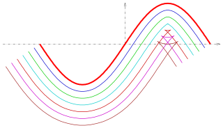
The B-spline basis functions used in the construction of NURBS curves are usually denoted as ${\displaystyle N_{i,n}(u)}$, in which ${\displaystyle i}$ corresponds to the ${\displaystyle i}$-th control point, and ${\displaystyle n}$ corresponds with the degree of the basis function. ^[11] The parameter dependence is frequently left out, so we can write ${\displaystyle N_{i,n}}$. The definition of these basis functions is recursive in ${\displaystyle n}$. The degree-0 functions ${\displaystyle N_{i,0}}$ are piecewise constant functions. They are one on the corresponding knot span and zero everywhere else. Effectively, ${\displaystyle N_{i,n}}$ is a linear interpolation of ${\displaystyle N_{i,n-1}}$ and ${\displaystyle N_{i+1,n-1}}$. The latter two functions are non-zero for ${\displaystyle n}$ knot spans, overlapping for ${\displaystyle n-1}$ knot spans. The function ${\displaystyle N_{i,n}}$ is computed as

From top to bottom: Linear basis functions ${\displaystyle N_{1,1}}$ (blue) and ${\displaystyle N_{2,1}}$ (green) (top), their weight functions ${\displaystyle f}$ and ${\displaystyle g}$ (middle) and the resulting quadratic basis function (bottom). The knots are 0, 1, 2, and 2.5

$${\displaystyle N_{i,n}=f_{i,n}N_{i,n-1}+g_{i+1,n}N_{i+1,n-1}}$$

${\displaystyle f_{i}}$ rises linearly from zero to one on the interval where ${\displaystyle N_{i,n-1}}$ is non-zero, while ${\displaystyle g_{i+1}}$ falls from one to zero on the interval where ${\displaystyle N_{i+1,n-1}}$ is non-zero. As mentioned before, ${\displaystyle N_{i,1}}$ is a triangular function, nonzero over two knot spans rising from zero to one on the first, and falling to zero on the second knot span. Higher order basis functions are non-zero over corresponding more knot spans and have correspondingly higher degree. If ${\displaystyle u}$ is the parameter, and ${\displaystyle k_{i}}$ is the ${\displaystyle i}$^th knot, we can write the functions ${\displaystyle f}$ and ${\displaystyle g}$ as

$${\displaystyle f_{i,n}(u)={\frac {u-k_{i}}{k_{i+n}-k_{i}}}}$$

and

$${\displaystyle g_{i,n}(u)=1-f_{i,n}(u)={\frac {k_{i+n}-u}{k_{i+n}-k_{i}}}}$$

The functions ${\displaystyle f}$ and ${\displaystyle g}$ are positive when the corresponding lower order basis functions are non-zero. By induction on n it follows that the basis functions are non-negative for all values of ${\displaystyle n}$ and ${\displaystyle u}$. This makes the computation of the basis functions numerically stable.

Again by induction, it can be proved that the sum of the basis functions for a particular value of the parameter is unity. This is known as the partition of unity property of the basis functions.

Linear basis functions

Quadratic basis functions

The figures show the linear and the quadratic basis functions for the knots {..., 0, 1, 2, 3, 4, 4.1, 5.1, 6.1, 7.1, ...}

One knot span is considerably shorter than the others. On that knot span, the peak in the quadratic basis function is more distinct, reaching almost one. Conversely, the adjoining basis functions fall to zero more quickly. In the geometrical interpretation, this means that the curve approaches the corresponding control point closely. In case of a double knot, the length of the knot span becomes zero and the peak reaches one exactly. The basis function is no longer differentiable at that point. The curve will have a sharp corner if the neighbour control points are not collinear.

General form of a NURBS curve

Using the definitions of the basis functions ${\displaystyle N_{i,n}}$ from the previous paragraph, a NURBS curve takes the following form: ^[11]

$${\displaystyle C(u)=\sum _{i=1}^{k}{\frac {N_{i,n}(u)w_{i}}{\sum _{j=1}^{k}N_{j,n}(u)w_{j}}}\mathbf {P} _{i}={\frac {\sum _{i=1}^{k}{N_{i,n}(u)w_{i}\mathbf {P} _{i}}}{\sum _{i=1}^{k}{N_{i,n}(u)w_{i}}}}}$$

In this, ${\displaystyle k}$ is the number of control points ${\displaystyle \mathbf {P} _{i}}$ and ${\displaystyle w_{i}}$ are the corresponding weights. The denominator is a normalizing factor that evaluates to one if all weights are one. This can be seen from the partition of unity property of the basis functions. It is customary to write this as

$${\displaystyle C(u)=\sum _{i=1}^{k}R_{i,n}(u)\mathbf {P} _{i}}$$

in which the functions

$${\displaystyle R_{i,n}(u)={N_{i,n}(u)w_{i} \over \sum _{j=1}^{k}N_{j,n}(u)w_{j}}}$$

are known as the rational basis functions.

General form of a NURBS surface

A NURBS surface is obtained as the tensor product of two NURBS curves, thus using two independent parameters ${\displaystyle u}$ and ${\displaystyle v}$ (with indices ${\displaystyle i}$ and ${\displaystyle j}$ respectively): ^[11]

$${\displaystyle S(u,v)=\sum _{i=1}^{k}\sum _{j=1}^{l}R_{i,j}(u,v)\mathbf {P} _{i,j}}$$

with

$${\displaystyle R_{i,j}(u,v)={\frac {N_{i,n}(u)N_{j,m}(v)w_{i,j}}{\sum _{p=1}^{k}\sum _{q=1}^{l}N_{p,n}(u)N_{q,m}(v)w_{p,q}}}}$$

as rational basis functions.

Manipulating NURBS objects

Motoryacht design using NURBS surfaces

A number of transformations can be applied to a NURBS object. For instance, if some curve is defined using a certain degree and N control points, the same curve can be expressed using the same degree and N+1 control points. In the process a number of control points change position and a knot is inserted in the knot vector. These manipulations are used extensively during interactive design. When adding a control point, the shape of the curve should stay the same, forming the starting point for further adjustments. A number of these operations are discussed below. ^{[11] [12]}

Knot insertion

As the term suggests, knot insertion inserts a knot into the knot vector. If the degree of the curve is ${\displaystyle n}$, then ${\displaystyle n-1}$ control points are replaced by ${\displaystyle n}$ new ones. The shape of the curve stays the same.

A knot can be inserted multiple times, up to the maximum multiplicity of the knot. This is sometimes referred to as knot refinement and can be achieved by an algorithm that is more efficient than repeated knot insertion.

Knot removal

Knot removal is the reverse of knot insertion. Its purpose is to remove knots and the associated control points in order to get a more compact representation. Obviously, this is not always possible while retaining the exact shape of the curve. In practice, a tolerance in the accuracy is used to determine whether a knot can be removed. The process is used to clean up after an interactive session in which control points may have been added manually, or after importing a curve from a different representation, where a straightforward conversion process leads to redundant control points.

Degree elevation

A NURBS curve of a particular degree can always be represented by a NURBS curve of higher degree. This is frequently used when combining separate NURBS curves, e.g., when creating a NURBS surface interpolating between a set of NURBS curves or when unifying adjacent curves. In the process, the different curves should be brought to the same degree, usually the maximum degree of the set of curves. The process is known as degree elevation.

Curvature

The most important property in differential geometry is the curvature ${\displaystyle \kappa }$. It describes the local properties (edges, corners, etc.) and relations between the first and second derivative, and thus, the precise curve shape. Having determined the derivatives it is easy to compute ${\displaystyle \kappa ={\frac {|r'(t)\times r''(t)|}{|r'(t)|^{3}}}}$ or approximated as the arclength from the second derivative ${\displaystyle \kappa =|r''(s_{o})|}$. The direct computation of the curvature ${\displaystyle \kappa }$ with these equations is the big advantage of parameterized curves against their polygonal representations.

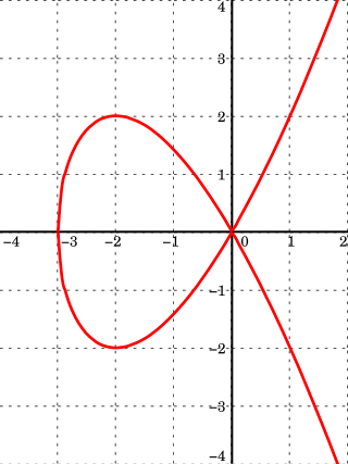
Example: a circle

NURBS have the ability to exactly describe circles. Here, the black triangle is the control polygon of a NURBS curve (shown at w=1). The Blue dotted line shows the corresponding control polygon of a B-spline curve in 3D homogeneous coordinates, formed by multiplying the NURBS by the control points by the corresponding weights. The blue parabolas are the corresponding B-spline curve in 3D, consisting of three parabolas. By choosing the NURBS control points and weights, the parabolas are parallel to the opposite face of the gray cone (with its tip at the 3D origin), so dividing by w to project the parabolas onto the w=1 plane results in circular arcs (red circle; see conic section).

Non-rational splines or Bézier curves may approximate a circle, but they cannot represent it exactly. Rational splines can represent any conic section—including the circle—exactly. This representation is not unique, but one possibility appears below:

x	y	z	Weight
1	0	0	1
1	1	0	${\displaystyle \scriptstyle {\frac {\sqrt {2}}{2}}}$
0	1	0	1
-1	1	0	${\displaystyle \scriptstyle {\frac {\sqrt {2}}{2}}}$
-1	0	0	1
-1	-1	0	${\displaystyle \scriptstyle {\frac {\sqrt {2}}{2}}}$
0	-1	0	1
1	-1	0	${\displaystyle \scriptstyle {\frac {\sqrt {2}}{2}}}$
1	0	0	1

The order is three, since a circle is a quadratic curve and the spline's order is one more than the degree of its piecewise polynomial segments. The knot vector is ${\displaystyle \{0,0,0,\pi /2,\pi /2,\pi ,\pi ,3\pi /2,3\pi /2,2\pi ,2\pi ,2\pi \}\,}$. The circle is composed of four quarter circles, tied together with double knots. Although double knots in a third order NURBS curve would normally result in loss of continuity in the first derivative, the control points are positioned in such a way that the first derivative is continuous. In fact, the curve is infinitely differentiable everywhere, as it must be if it exactly represents a circle.

The curve represents a circle exactly, but it is not exactly parametrized in the circle's arc length. This means, for example, that the point at ${\displaystyle t}$ does not lie at ${\displaystyle (\sin(t),\cos(t))}$ (except for the start, middle and end point of each quarter circle, since the representation is symmetrical). This would be impossible, since the x coordinate of the circle would provide an exact rational polynomial expression for ${\displaystyle \cos(t)}$, which is impossible. The circle does make one full revolution as its parameter ${\displaystyle t}$ goes from 0 to ${\displaystyle 2\pi }$, but this is only because the knot vector was arbitrarily chosen as multiples of ${\displaystyle \pi /2}$.

See also

• Spline
• Bézier surface
• de Boor's algorithm
• Triangle mesh
• Point cloud
• Rational motion
• Isogeometric analysis

References

1. https://www.willgibbons.com/rendering-software/
2. Schneider, Philip. "NURB Curves: A Guide for the Uninitiated". MACTECH. Retrieved 26 September 2014.
3. Schneider, Philip (March 1996). "NURB Curves: A Guide for the Uninitiated" (PDF). develop (25): 48–74.
4. Schoenberg, I. J. (August 19, 1964). "Spline Functions and the Problem of Graduation". Proceedings of the National Academy of Sciences of the United States of America . 52 (4). National Academy of Sciences: 947–950. Bibcode:1964PNAS...52..947S. doi: 10.1073/pnas.52.4.947 . PMC   300377 . PMID   16591233.
5. Foley, van Dam, Feiner & Hughes: Computer Graphics: Principles and Practice , section 11.2, Addison-Wesley 1996 (2nd ed.).
6. Bio-Inspired Self-Organizing Robotic Systems. p. 9. Retrieved 2014-01-06.
7. "Rational B-splines". www.cl.cam.ac.uk.
8. "NURBS: Definition". www.cs.mtu.edu.
9. David F. Rogers: An Introduction to NURBS with Historical Perspective, section 7.1
10. Gershenfeld, Neil (1999). The Nature of Mathematical Modeling. Cambridge University Press. p. 141. ISBN   0-521-57095-6.
11. Piegl, Les; Tiller, Wayne (1997). The NURBS Book (2. ed.). Berlin: Springer. ISBN   3-540-61545-8.
12. Piegl, L. (1989). "Modifying the shape of rational B-splines. Part 1: curves". Computer-Aided Design. 21 (8): 509–518. doi:10.1016/0010-4485(89)90059-6.

External links

• Clear explanation of NURBS for non-experts
• About Nonuniform Rational B-Splines – NURBS
• TinySpline: Opensource C-library with bindings for various languages