Pulse compression

Pulse compression is a signal processing technique commonly used by radar, sonar and echography to either increase the range resolution when pulse length is constrained or increase the signal to noise ratio when the peak power and the bandwidth (or equivalently range resolution) of the transmitted signal are constrained. This is achieved by modulating the transmitted pulse and then correlating the received signal with the transmitted pulse. ^[1]

Simple pulse

Signal description

The ideal model for the simplest, and historically first type of signals a pulse radar or sonar can transmit is a truncated sinusoidal pulse (also called a CW --carrier wave-- pulse), of amplitude ${\displaystyle A}$ and carrier frequency, ${\displaystyle f_{0}}$, truncated by a rectangular function of width, ${\displaystyle T}$. The pulse is transmitted periodically, but that is not the main topic of this article; we will consider only a single pulse, ${\displaystyle s}$. If we assume the pulse to start at time ${\displaystyle t=0}$, the signal can be written the following way, using the complex notation:

${\displaystyle s(t)={\begin{cases}e^{2i\pi f_{0}t}&{\text{if}}\;0\leq t<T\\0&{\text{otherwise}}\end{cases}}}$

Range resolution

Let us determine the range resolution which can be obtained with such a signal. The return signal, written ${\displaystyle r(t)}$, is an attenuated and time-shifted copy of the original transmitted signal (in reality, Doppler effect can play a role too, but this is not important here.) There is also noise in the incoming signal, both on the imaginary and the real channel. The noise is assumed to be band-limited, that is to have frequencies only in ${\displaystyle [f_{0}-\Delta f/2,f_{0}+\Delta f/2]}$ (this generally holds in reality, where a bandpass filter is generally used as one of the first stages in the reception chain); we write ${\displaystyle N(t)}$ to denote that noise. To detect the incoming signal, a matched filter is commonly used. This method is optimal when a known signal is to be detected among additive noise having a normal distribution.

In other words, the cross-correlation of the received signal with the transmitted signal is computed. This is achieved by convolving the incoming signal with a conjugated and time-reversed version of the transmitted signal. This operation can be done either in software or with hardware. We write ${\displaystyle \langle s,r\rangle (t)}$ for this cross-correlation. We have:

${\displaystyle \langle s,r\rangle (t)=\int _{t'\,=\,0}^{+\infty }s^{\star }(t')r(t+t')dt'}$

If the reflected signal comes back to the receiver at time ${\displaystyle t_{r}}$ and is attenuated by factor ${\displaystyle A}$, this yields:

${\displaystyle r(t)=\left\{{\begin{array}{ll}Ae^{2i\pi f_{0}(t\,-\,t_{r})}+N(t)&{\mbox{if}}\;t_{r}\leq t<t_{r}+T\\N(t)&{\mbox{otherwise}}\end{array}}\right.}$

Since we know the transmitted signal, we obtain:

${\displaystyle \langle s,r\rangle (t)=A\Lambda \left({\frac {t-t_{r}}{T}}\right)e^{2i\pi f_{0}(t\,-\,t_{r})}+N'(t)}$

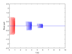
where ${\displaystyle N'(t)}$, is the result of the intercorrelation between the noise and the transmitted signal. Function ${\displaystyle \Lambda }$ is the triangle function, its value is 0 on ${\textstyle [-\infty ,-{\frac {1}{2}}]\cup [{\frac {1}{2}},+\infty ]}$, it increases linearly on ${\textstyle [-{\frac {1}{2}},0]}$ where it reaches its maximum 1, and it decreases linearly on ${\textstyle [0,{\frac {1}{2}}]}$ until it reaches 0 again. Figures at the end of this paragraph show the shape of the intercorrelation for a sample signal (in red), in this case a real truncated sine, of duration ${\displaystyle T=1}$ seconds, of unit amplitude, and frequency ${\textstyle f_{0}=10}$ hertz. Two echoes (in blue) come back with delays of 3 and 5 seconds and amplitudes equal to 0.5 and 0.3 times the amplitude of the transmitted pulse, respectively; these are just random values for the sake of the example. Since the signal is real, the intercorrelation is weighted by an additional 1⁄2 factor.

If two pulses come back (nearly) at the same time, the intercorrelation is equal to the sum of the intercorrelations of the two elementary signals. To distinguish one "triangular" envelope from that of the other pulse, it is clearly visible that the times of arrival of the two pulses must be separated by at least ${\displaystyle T}$ so that the maxima of both pulses can be separated. If this condition is not met, both triangles will be mixed together and impossible to separate.

Since the distance travelled by a wave during ${\displaystyle T}$ is ${\displaystyle cT}$ (where c is the speed of the wave in the medium), and since this distance corresponds to a round-trip time, we get:

Result 1
The range resolution with a sinusoidal pulse is ${\textstyle {\frac {1}{2}}cT}$ where ${\displaystyle T}$ is the pulse Duration and, ${\displaystyle c}$, the speed of the wave. Conclusion: to increase the resolution, the pulse length must be reduced.

 

Example (simple impulsion): transmitted signal in red (carrier 10 hertz, amplitude 1, duration 1 second) and two echoes (in blue).

Before matched filtering	After matched filtering
If the targets are separated enough...	...echoes can be distinguished.
If the targets are too close...	...the echoes are mixed together.

Energy and signal-to-noise ratio of the received signal

The instantaneous power of the received pulse is ${\displaystyle P(t)=|r|^{2}(t)}$. The energy put into that signal is:

${\displaystyle E=\int _{0}^{T}P(t)dt=A^{2}T}$

If ${\displaystyle \sigma }$ is the standard deviation of the noise which is assumed to have the same bandwidth as the signal, the signal-to-noise ratio (SNR) at the receiver is:

${\displaystyle SNR={\frac {E_{r}}{\sigma ^{2}}}={\frac {A^{2}T}{\sigma ^{2}}}}$

The SNR is proportional to pulse duration ${\displaystyle T}$, if other parameters are held constant. This introduces a tradeoff: increasing ${\displaystyle T}$ improves the SNR, but reduces the resolution, and vice versa.

Pulse compression by linear frequency modulation (or chirping)

Basic principles

How can one have a large enough pulse (to still have a good SNR at the receiver) without poor resolution? This is where pulse compression enters the picture. The basic principle is the following:

• a signal is transmitted, with a long enough length so that the energy budget is correct
• this signal is designed so that after matched filtering, the width of the intercorrelated signals is smaller than the width obtained by the standard sinusoidal pulse, as explained above (hence the name of the technique: pulse compression).

In radar or sonar applications, linear chirps are the most typically used signals to achieve pulse compression. The pulse being of finite length, the amplitude is a rectangle function. If the transmitted signal has a duration ${\displaystyle T}$, begins at ${\displaystyle t=0}$ and linearly sweeps the frequency band ${\displaystyle \Delta f}$ centered on carrier ${\displaystyle f_{0}}$, it can be written:

${\displaystyle s_{c}(t)=\left\{{\begin{array}{ll}e^{i2\pi \left(\left(f_{0}\,-\,{\frac {\Delta f}{2}}\right)t\,+\,{\frac {\Delta f}{2T}}t^{2}\,\right)}&{\mbox{if}}\;0\leq t<T\\0&{\mbox{otherwise}}\end{array}}\right.}$

The chirp definition above means that the phase of the chirped signal (that is, the argument of the complex exponential), is the quadratic:

${\displaystyle \phi (t)=2\pi \left(\left(f_{0}\,-\,{\frac {\Delta f}{2}}\right)t\,+\,{\frac {\Delta f}{2T}}t^{2}\,\right)}$

thus the instantaneous frequency is (by definition):

${\displaystyle f(t)={\frac {1}{2\pi }}\left[{\frac {d\phi }{dt}}\right]_{t}=f_{0}-{\frac {\Delta f}{2}}+{\frac {\Delta f}{T}}t}$

which is the intended linear ramp going from ${\displaystyle f_{0}-{\frac {\Delta f}{2}}}$ at ${\displaystyle t=0}$ to ${\textstyle f_{0}+{\frac {\Delta f}{2}}}$ at ${\displaystyle t=T}$.

The relation of phase to frequency is often used in the other direction, starting with the desired ${\displaystyle f(t)}$ and writing the chirp phase via the integration of frequency:

${\displaystyle \phi (t)=2\pi \int _{0}^{t}f(u)\,du}$

This transmitted signal is typically reflected by the target and undergoes attenuation due to various causes, so the received signal is a time-delayed, attenuated version of the transmitted signal plus an additive noise of constant power spectral density on ${\displaystyle [f_{0}-\Delta f/2,f_{0}+\Delta f/2]}$, and zero everywhere else:

${\displaystyle r(t)=\left\{{\begin{array}{ll}Ae^{i2\pi \left(\left(f_{0}\,-\,{\frac {\Delta f}{2}}\right)(t-t_{r})\,+\,{\frac {\Delta f}{2T}}(t-t_{r})^{2}\,\right)}+N(t)&{\mbox{if}}\;t_{r}\leq t<t_{r}+T\\N(t)&{\mbox{otherwise}}\end{array}}\right.}$

Cross-correlation between the transmitted and the received signal

We now endeavor to compute the correlation of the received signal with the transmitted signals. Two actions are going to be taken to do this:

- The first action is a simplification. Instead of computing the cross-correlation we are going to compute an auto-correlation which amounts to assuming that the autocorrelation peak is centered at zero. This will not change the resolution and the amplitudes but will simplify the math:

${\displaystyle r'(t)={\begin{cases}Ae^{2i\pi \left(f_{0}\,+\,{\frac {\Delta f}{2T}}t\right)t}+N(t)&{\mbox{if}}\;-{\frac {T}{2}}\leq t<{\frac {T}{2}}\\N(t)&{\mbox{otherwise}}\end{cases}}}$

- The second action is, as shown below, is to set an amplitude for the reference signal which is not one, but ${\displaystyle \rho \neq 1}$. Constant ${\displaystyle \rho }$ is to be determined so that energy is conserved through correlation.

${\displaystyle s_{c}'(t)={\begin{cases}\rho e^{2i\pi \left(f_{0}\,+\,{\frac {\Delta f}{2T}}t\right)t}&{\mbox{if}}\;-{\frac {T}{2}}\leq t<{\frac {T}{2}}\\0&{\mbox{otherwise}}\end{cases}}}$

Now, it can be shown ^[2] that the correlation function of ${\displaystyle s_{c}'}$ with ${\displaystyle r'}$ is:

${\displaystyle \langle s_{c}',r'\rangle (t)=\rho A{\sqrt {T}}\Lambda \left({\frac {t}{T}}\right)\mathrm {sinc} \left[\Delta ft\Lambda \left({\frac {t}{T}}\right)\right]e^{2i\pi f_{0}t}+N'(t)}$

where ${\displaystyle N'(t)}$ is the correlation of the reference signal with the received noise.

Width of the signal after correlation

Assuming noise is zero, the maximum of the autocorrelation function of ${\displaystyle s_{c'}}$ is reached at 0. Around 0, this function behaves as the sinc (or cardinal sine) term, defined here as ${\displaystyle sinc(x)=sin(\pi x)/(\pi x)}$. The −3 dB temporal width of that cardinal sine is more or less equal to ${\textstyle T'={\frac {1}{\Delta f}}}$. Everything happens as if, after matched filtering, we had the resolution that would have been reached with a simple pulse of duration ${\displaystyle T'}$. For the common values of ${\displaystyle \Delta f}$, ${\displaystyle T'}$ is smaller than ${\displaystyle T}$, hence the pulse compression name.

Since the cardinal sine can have annoying sidelobes, a common practice is to filter the result by a window (Hamming, Hann, etc.). In practice, this can be done at the same time as the adapted filtering by multiplying the reference chirp with the filter. The result will be a signal with a slightly lower maximum amplitude, but the sidelobes will be filtered out, which is more important.

Result 2
The distance resolution reachable with a linear frequency modulation of a pulse on a bandwidth ${\displaystyle \Delta f}$ is: ${\textstyle {\frac {c}{2\Delta f}}}$ where ${\displaystyle c}$ is the speed of the wave.

 

Definition
Ratio ${\textstyle {\frac {T}{T'}}=T\Delta f}$ is the pulse compression ratio. It is generally greater than 1 (usually, its value is 20 to 30).

 

Example (chirped pulse): transmitted signal in red (carrier 10 hertz, modulation on 16 hertz, amplitude 1, duration 1 second) and two echoes (in blue).

Before matched filtering: the echoes are long and have a low amplitude

After matched filtering: the echoes are shorter in time and have a higher peak power.

Energy and peak power after correlation

When the reference signal ${\displaystyle s_{c}'}$ is correctly scaled using term ${\displaystyle \rho }$, then it is possible to conserve the energy before and after correlation. The peak (and average) power before correlation is:

${\displaystyle P_{r'}=|r'(t)|^{2}=P_{r'}^{peak}=A^{2}}$

Since, before compression, the pulse is box-shaped, the energy before correlation is:

${\displaystyle E_{r'}=\int _{-T/2}^{T/2}|r'(t)|^{2}dt=A^{2}T}$

The peak power after correlation is reached at ${\displaystyle t=0}$:

${\displaystyle P_{<s_{c}',r'>}^{peak}=|<s_{c}',r'>(0)|^{2}=\rho ^{2}A^{2}T}$

Note that if ${\displaystyle \rho =1}$ this peak power is the energy of the received signal before correlation, which is as expected. After compression, the pulse is approximal by a box having a width equal to the typical width of the ${\displaystyle sinc}$ function, that is, a width ${\displaystyle T'=1/\Delta f}$, so the energy after correlation is:

${\displaystyle E_{<s_{c}',r'>}=\int _{-\infty }^{+\infty }|<s_{c}',r'>(t)|^{2}dt\approx P_{<s_{c}',r'>}^{peak}\times T'=\rho ^{2}{\frac {A^{2}T}{\Delta f}}}$

If energy is conserved:

${\displaystyle E_{r'}=E_{<s_{c}',r'>}}$

... it comes that: ${\displaystyle \rho ={\sqrt {\Delta f}}}$ so that the peak power after correlation is:

${\displaystyle P_{<s_{c}',r'>}^{peak}=\rho ^{2}A^{2}T=P_{r'}\times \Delta f\times T}$

As a conclusion, the peak power of the pulse-compressed signal is ${\displaystyle \Delta f\times T}$ that of the raw received signal (assuming that the template ${\displaystyle s_{c}'}$ is correctly scaled to conserve energy through correlation).

Signal-to-noise gain after correlation

Equivalence between a chirped pulse and a shorter CW pulse after pulse compression. Energy is the area under the blue curves (in the time domain); power is the area under the red curves (in the spectral domain).

As we have seen above, things are written so that the energy of the signal does not vary during pulse compression. However, it is now located in the main lobe of the cardinal sine, whose width is approximately ${\textstyle T'\approx {\frac {1}{\Delta f}}}$. If ${\displaystyle P}$ is the power of the signal before compression, and ${\displaystyle P'}$ the power of the signal after compression, energy ${\displaystyle E}$ is conserved and we have:

${\displaystyle E=P\times T=P'\times T'}$

which yields an increase in power after pulse compression:

${\displaystyle P'=P\times {\frac {T}{T'}}}$

In the spectral domain, the power spectrum of the chirp has a nearly constant spectral density ${\displaystyle D=P/\Delta f}$ in interval ${\displaystyle [f_{0}-\Delta f/2,f_{0}+\Delta f/2]}$ and zero elsewhere, so that energy is equivalently expressed as ${\displaystyle E=P\times T=D.\Delta f.T}$. This spectral density remains the same after matched filtering.

Imagining now an equivalent sinusoidal (CW) pulse of duration ${\displaystyle T'=1/\Delta f}$ and identical input power, this equivalent sinusoidal pulse has an energy:

${\displaystyle E'=P\times T'=E{\frac {T'}{T}}}$

After matched filtering, the equivalent sinusoidal pulse turns into a triangular-shaped signal of twice its original width but the same peak power. Energy is conserved. The spectral domain is approximated by a nearly constant spectral density ${\displaystyle D'}$ in interval ${\displaystyle [f_{0}-\Delta f/2,f_{0}+\Delta f/2]}$ where ${\displaystyle \Delta f\approx 1/T'}$. Through conservation of energy, we have:

${\displaystyle E'=E{\frac {T'}{T}}=D\Delta fT{\frac {T'}{T}}=D\Delta fT'}$

Since by definition we also have: ${\displaystyle E'=D'\Delta fT'}$ it comes that: ${\displaystyle D'=D}$ meaning that the spectral densities of the chirped pulse, and the equivalent CW pulse are very nearly identical, and are equivalent to that of a bandpass filter on ${\displaystyle [f_{0}-\Delta f/2,f_{0}+\Delta f/2]}$. The filtering effect of correlation also acts on the noise, meaning that the reference band for the noise is ${\displaystyle \Delta f}$ and since ${\displaystyle D=D'}$, the same filtering effect is obtained on the noise in both cases after correlation. This means that the net effect of pulse compression is that, compared to the equivalent CW pulse, the signal-to-noise ratio (SNR) has improved by a factor ${\displaystyle T/T'}$ because the signal is amplified but not the noise.

As a consequence:  

Result 3

After pulse compression, the signal-to-noise ratio can be considered as being amplified by ${\displaystyle T\Delta f}$as compared to the baseline situation of a continuous-wave pulse of duration ${\displaystyle T'=1/\Delta f}$ and the same amplitude as the chirp-modulated signal before compression, where the received signal and noise have (implicitly) undergone a bandpass filtering on ${\displaystyle [f_{0}-\Delta f/2,f_{0}+\Delta f/2]}$. This additional gain can be injected into the radar equation.

 

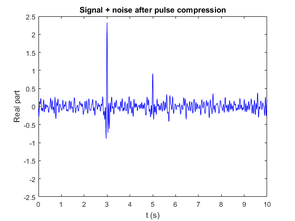
Example: same signals as above, plus an additive white Gaussian having undergone bandpass filtering (standard deviation of real part: 0.125 after filtering). After correlation, the power of the noise is unchanged. The signal itself is amplified by a factor four (or 16 for the power, as predicted by theory).

Before matched filtering: the signal is hidden in noise

After matched filtering: echoes become visible.

For technical reasons, correlation is not necessarily done for actual received CW pulses as for chirped pulses. However during baseband shifting the signal undergoes a bandpass filtering on ${\displaystyle [f_{0}-\Delta f/2,f_{0}+\Delta f/2]}$ which has the same net effect on the noise as the correlation, so the overall reasoning remains the same (that is, the SNR makes only sense for noise defined on a given bandwidth, here being that of the signal).

This gain in the SNR seems magical, but remember that the power spectral density does not represent the phase of the signal. In reality the phases are different for the equivalent CW pulse, the CW pulse after correlation, the original chirped pulse and the correlated chirped pulse, which explains the different shapes of the signals (especially the varying lengths) despite having (nearly) the same power spectrum in all cases. If the peak transmitting power ${\displaystyle P}$ and the bandwidth ${\displaystyle \Delta f}$ are constrained, pulse compression thus achieves a better peak power (but same resolution) by transmitting a longer pulse (that is, more energy), compared to an equivalent CW pulse of same peak power ${\displaystyle P}$ and bandwidth ${\displaystyle \Delta f}$, and squeezing the pulse by correlation. This works best only for a limited number of signal types which, after correlation, have a narrower peak than the original signal, and low sidelobes.

Stretch processing

While pulse compression can ensure good SNR and fine range resolution in the same time, digital signal processing in such a system can be difficult to implement because of the high instantaneous bandwidth of the waveform (${\displaystyle \Delta f}$ can be hundreds of megahertz or even exceed 1 GHz.) Stretch Processing is a technique for matched filtering of wideband chirping waveform and is suitable for applications seeking very fine range resolution over relatively short range intervals. ^[3]

Stretch processing

Picture above shows the scenario for analyzing stretch processing. The central reference point(CRP) is in the middle of the range window of interest at range of ${\displaystyle R_{0}}$, corresponding to a time delay of ${\displaystyle t_{0}}$.

If the transmitted waveform is the chirp waveform:

${\displaystyle x(t)=\exp \left(j\pi {\frac {\Delta f}{T}}(t)^{2}\right)\exp(j2\pi f_{0}(t)),0\leq t\leq T}$

then the echo from the target at distance ${\displaystyle R_{b}}$can be expressed as:

${\displaystyle {\bar {x}}(t)=\rho \exp \left(j\pi {\frac {\Delta f}{T}}(t-t_{b})^{2}\right)\exp(j2\pi f_{0}(t-t_{b})),0\leq t-t_{b}\leq T}$

where ${\displaystyle \rho }$ is proportional to the scatterer reflectivity. We then multiply the echo by ${\textstyle \exp(-j2\pi f_{0}t)\exp \left(-j\pi {\frac {\Delta f}{T}}(t-t_{0})^{2}\right)}$ and the echo will become:

${\displaystyle y(t)=\rho \exp \left(-j{\frac {4\pi R_{b}}{\lambda }}\right)\exp \left(-j2\pi {\frac {\Delta f}{T}}\delta t_{b}(t-t_{0})\right)\exp \left(j\pi {\frac {\Delta f}{T}}(\delta t_{b})^{2}\right),t_{0}\leq t-\delta t_{b}\leq t_{0}+T}$

where ${\displaystyle \lambda }$ is the wavelength of electromagnetic wave in air.

After conducting sampling and discrete Fourier transform on y(t) the sinusoid frequency ${\displaystyle F_{b}}$ can be solved:

${\displaystyle F_{b}=-\delta t_{b}{\frac {\Delta f}{T}}(Hz)}$

and the differential range ${\displaystyle \delta R_{b}}$ can be obtained:

${\displaystyle \delta R_{b}=-{\frac {cTF_{b}}{2\Delta f}}}$

To show that the bandwidth of y(t) is less than the original signal bandwidth ${\displaystyle \Delta f}$, we suppose that the range window is ${\displaystyle R_{w}={\frac {cT_{w}}{2}}}$ long. If the target is at the lower bound of the range window, the echo will arrive ${\displaystyle t_{0}-T_{w}/2}$ seconds after transmission; similarly, If the target is at the upper bound of the range window, the echo will arrive ${\displaystyle t_{0}+T_{w}/2}$ seconds after transmission. The differential arrive time ${\displaystyle \delta t_{b}}$ for each case is ${\displaystyle -T_{w}/2}$ and ${\displaystyle T_{w}/2}$, respectively.

We can then obtain the bandwidth by considering the difference in sinusoid frequency for targets at the lower and upper bound of the range window:

$${\displaystyle \Delta f_{s}=F_{b,{\text{near}}}-F_{b,{\text{far}}}=-{\frac {\Delta f}{T}}(-T_{w}/2-T_{w}/2)={\frac {T_{w}}{T}}\Delta f}$$

As a consequence:  

Result 4
Through stretch processing, the bandwidth at the receiver output is less than the original signal bandwidth if ${\displaystyle T_{w}<T}$, thereby facilitating the implementation of DSP system in a linear-frequency-modulation radar system.

  To demonstrate that stretch processing preserves range resolution, we need to understand that y(t) is actually an impulse train with pulse duration T and period ${\displaystyle T_{trans}}$, which is equal to the period of the transmitted impulse train. As a result, the Fourier transform of y(t) is actually a sinc function with Rayleigh resolution ${\textstyle {\frac {1}{T}}}$. That is, the processor will be able to resolve scatterers whose ${\displaystyle F_{b}}$ are at least ${\displaystyle \Delta F_{b}=1/T}$ apart.

Consequently,

${\displaystyle {\frac {1}{T}}=\left\vert {\frac {\Delta f}{T}}\Delta (\delta t_{b})\right\vert \Rightarrow \left\vert \Delta (\delta t_{b})\right\vert ={\frac {1}{\Delta f}}}$

and,

${\displaystyle \Delta (\delta R_{b})={\frac {c\Delta (\delta t_{b})}{2}}={\frac {c}{2\Delta f}}}$

which is the same as the resolution of the original linear frequency modulation waveform.

Stepped-frequency waveform

Although stretch processing can reduce the bandwidth of received baseband signal, all of the analog components in RF front-end circuitry still must be able to support an instantaneous bandwidth of ${\displaystyle \Delta f}$. In addition, the effective wavelength of the electromagnetic wave changes during the frequency sweep of a chirp signal, and therefore the antenna look direction will be inevitably changed in a Phased array system.

Stepped-frequency waveforms are an alternative technique that can preserve fine range resolution and SNR of the received signal without large instantaneous bandwidth. Unlike the chirping waveform, which sweeps linearly across a total bandwidth of ${\displaystyle \Delta f}$ in a single pulse, stepped-frequency waveform employs an impulse train where the frequency of each pulse is increased by ${\displaystyle \Delta F}$ from the preceding pulse. The baseband signal can be expressed as:

${\displaystyle x(t)=\sum _{m=0}^{M-1}x_{p}(t-mT)e^{j2\pi m\Delta F(t-mT)}}$

where ${\displaystyle x_{p}(t)}$ is a rectangular impulse of length ${\displaystyle \tau }$ and M is the number of pulses in a single pulse train. The total bandwidth of the waveform is still equal to ${\displaystyle \Delta f=M\Delta F}$, but the analog components can be reset to support the frequency of the following pulse during the time between pulses. As a result, the problem mentioned above can be avoided.

To calculate the distance of the target corresponding to a delay ${\displaystyle t_{l}+\delta t}$, individual pulses are processed through the simple pulse matched filter:

${\displaystyle h_{p}(t)=x_{p}^{*}(-t)}$

and the output of the matched filter is:

${\displaystyle y_{m}(t)=s_{p}^{*}(t-(t_{l}+\delta t)-mT)e^{j2\pi m\Delta F(t-(t_{l}+\delta t)-mT)}}$

where

${\displaystyle s_{p}^{*}(t-(t_{l}+\delta t)-mT)=x_{p}(t-(t_{l}+\delta t)-mT)*h_{p}(t)}$

If we sample ${\displaystyle y_{m}(t)}$ at ${\displaystyle t=t_{l}+mT}$, we can get:

${\displaystyle y[l,m]=s_{p}^{*}(\delta t)e^{j2\pi m\Delta F\delta t}}$

where l means the range bin l. Conduct DTFT (m is served as time here) and we can get:

${\displaystyle Y[l,\omega ]=\sum _{m=0}^{M-1}y[l,m]e^{-j\omega m}=s_{p}^{*}(\delta t)\sum _{m=0}^{M-1}e^{j(\omega -2\pi \Delta F\delta t)m}}$

,and the peak of the summation occurs when ${\displaystyle \omega =2\pi \Delta F\delta t}$.

Consequently, the DTFT of ${\displaystyle y[l,m]}$ provides a measure of the delay of the target relative to the range bin delay ${\displaystyle t_{l}}$:

$${\displaystyle \delta t={\frac {\omega _{p}}{2\pi \Delta F}}={\frac {f_{p}}{\Delta F}}}$$

and the differential range can be obtained:

${\displaystyle \delta R={\frac {cf_{p}}{2\Delta F}}}$

where c is the speed of light.

To demonstrate stepped-frequency waveform preserves range resolution, it should be noticed that ${\displaystyle Y[l,\omega ]}$ is a sinc-like function, and therefore it has a Rayleigh resolution of ${\displaystyle \Delta f_{p}=1/M}$. As a result:

${\displaystyle \Delta (\delta t)={\frac {1}{M\Delta F}}={\frac {1}{\Delta f}}}$

and therefore the differential range resolution is :

${\displaystyle \Delta (\delta R)={\frac {c}{2\Delta f}}}$

which is the same of the resolution of the original linear-frequency-modulation waveform.

Pulse compression by phase coding

There are other means to modulate the signal. Phase modulation is a commonly used technique; in this case, the pulse is divided in ${\displaystyle N}$ time slots of duration ${\textstyle {\frac {T}{N}}}$ for which the phase at the origin is chosen according to a pre-established convention. For instance, it is possible to not change the phase for some time slots (which comes down to just leaving the signal as it is, in those slots) and de-phase the signal in the other slots by ${\displaystyle \pi }$ (which is equivalent of changing the sign of the signal); this is known as binary phase-shift keying. The precise way of choosing the sequence of ${\displaystyle \{0,\pi \}}$ phases can be done according to a technique known as Barker codes.

The advantages ^[4] of the Barker codes are their simplicity (as indicated above, a ${\displaystyle \pi }$ de-phasing is a simple sign change), but the pulse compression ratio is lower than in the chirp case and the compression is very sensitive to frequency changes due to the Doppler effect if that change is larger than ${\textstyle {\frac {1}{T}}}$.

Other pseudorandom binary sequences have nearly optimal pulse compression properties, such as Gold codes, JPL codes or Kasami codes, because their autocorrelation peak is very narrow. These sequences have other interesting properties making them suitable for GNSS positioning, for instance.

It is possible to code the sequence on more than two phases (polyphase coding). As with a linear chirp, pulse compression is achieved through intercorrelation.

See also

• Continuous-wave radar
• Spread spectrum
• Chirp compression

Notes

1. J. R. Klauder, A. C, Price, S. Darlington and W. J. Albersheim, ‘The Theory and Design of Chirp Radars,” Bell System Technical Journal 39, 745 (1960).
2. Achim Hein, Processing of SAR Data: Fundamentals, Signal Processing, Interferometry, Springer, 2004, ISBN   3-540-05043-4, pages 38 to 44. Very rigorous demonstration of the autocorrelation function of a chirp. The author works with real chirps, hence the factor of 1⁄2 in his book, which is not used here.
3. Richards, Mark A. 2014. Fundamentals of radar signal processing. New York [etc.]: McGraw-Hill Education.
4. J.-P. Hardange, P. Lacomme, J.-C. Marchais, Radars aéroportés et spatiaux, Masson, Paris, 1995, ISBN   2-225-84802-5, page 104. Available in English: Air and Spaceborne Radar Systems: an introduction, Institute of Electrical Engineers, 2001, ISBN   0-85296-981-3

Further reading

• Nadav Levanon, and Eli Mozeson. Radar signals. Wiley. com, 2004.
• Hao He, Jian Li, and Petre Stoica. Waveform design for active sensing systems: a computational approach. Cambridge University Press, 2012.
• M. Soltanalian. Signal Design for Active Sensing and Communications. Uppsala Dissertations from the Faculty of Science and Technology (printed by Elanders Sverige AB), 2014.
• Solomon W. Golomb, and Guang Gong. Signal design for good correlation: for wireless communication, cryptography, and radar. Cambridge University Press, 2005.
• Fulvio Gini, Antonio De Maio, and Lee Patton, eds. Waveform design and diversity for advanced radar systems. Institution of engineering and technology, 2012.
• John J. Benedetto, Ioannis Konstantinidis, and Muralidhar Rangaswamy. "Phase-coded waveforms and their design." IEEE Signal Processing Magazine, 26.1 (2009): 22-31.
• Ducoff, Michael R., and Byron W. Tietjen. "Pulse compression radar." Radar Handbook (2008): 8-3.