Representative layer theory

Last updated

The concept of the representative layer came about though the work of Donald Dahm, with the assistance of Kevin Dahm and Karl Norris, to describe spectroscopic properties of particulate samples, especially as applied to near-infrared spectroscopy. [1] [2] A representative layer has the same void fraction as the sample it represents and each particle type in the sample has the same volume fraction and surface area fraction as does the sample as a whole. The spectroscopic properties of a representative layer can be derived from the spectroscopic properties of particles, which may be determined by a wide variety of ways. [3] While a representative layer could be used in any theory that relies on the mathematics of plane parallel layers, there is a set of definitions and mathematics, some old and some new, which have become part of representative layer theory.

Contents

Representative layer theory can be used to determine the spectroscopic properties of an assembly of particles from those of the individual particles in the assembly. [4] The sample is modeled as a series of layers, each of which is parallel to each other and perpendicular to the incident beam. The mathematics of plane parallel layers is then used to extract the desired properties from the data, most notably that of the linear absorption coefficient which behaves in the manner of the coefficient in Beer’s law. The representative layer theory gives a way of performing the calculations for new sample properties by changing the properties of a single layer of the particles, which doesn’t require reworking the mathematics for a sample as a whole.

History

The first attempt to account for transmission and reflection of a layered material was carried out by George G. Stokes in about 1860 [5] and led to some very useful relationships. John W. Strutt (Lord Rayleigh) [6] and Gustav Mie [7] developed the theory of single scatter to a high degree, but Aurthur Schuster [8] was the first to consider multiple scatter. He was concerned with the cloudy atmospheres of stars, and developed a plane-parallel layer model in which the radiation field was divided into forward and backward components. This same model was used much later by Paul Kubelka and Franz Munk, whose names are usually attached to it by spectroscopists.

Following WWII, the field of reflectance spectroscopy was heavily researched, both theoretically and experimentally.  The remission function, , following Kubelka-Munk theory, was the leading contender as the metric of absorption analogous to the absorbance function in transmission absorption spectroscopy. 

The form of the K-M solution originally was: , but it was rewritten in terms of linear coefficients by some authors, becoming , taking and as being equivalent to the linear absorption and scattering coefficients as they appear in the Bouguer-Lambert law, even though sources who derived the equations preferred the symbolism and usually emphasized that and was a remission or back-scattering parameter, which for the case of diffuse scatter should properly be taken as an integral. [9]

In 1966, in a book entitled Reflectance Spectroscopy, Harry Hecht had pointed out that the formulation led to , which enabled plotting "against the wavelength or wave-number for a particular sample" giving a curve corresponding "to the real absorption determined by transmission measurements, except for a displacement by in the ordinate direction." However, in data presented, "the marked deviation in the remission function ... in the region of large extinction is obvious." He listed various reasons given by other authors for this "failure ... to remain valid in strongly absorbing materials", including: "incomplete diffusion in the scattering process"; failure to use "diffuse illumination; "increased proportion of regular reflection"; but concluded that "notwithstanding the above mentioned difficulties, ... the remission function should be a linear function of the concentration at a given wavelength for a constant particle size" though stating that "this discussion has been restricted entirely to the reflectance of homogeneous powder layers" though "equation systems for combination of inhomogeneous layers cannot be solved for the scattering and absorbing properties even in the simple case of a dual combination of sublayers. ... This means that the (Kubelka-Munk) theory fails to include, in an explicit manner, any dependence of reflection on particle size or shape or refractive index". [10]

The field of Near infrared spectroscopy (NIR) got its start in 1968, when Karl Norris and co-workers with the Instrumentation Research Lab of the U.S. Department of Agriculture first applied the technology to agricultural products. [11] The USDA discovered how to use NIR empirically, based on available sources, gratings, and detector materials. Even the wavelength range of NIR was empirically set based on the operational range of a PbS detector. Consequently, it was not seen as a rigorous science: it had not evolved in the usual way, from research institutions to general usage. [12] Even though the Kubelka-Munk theory provided a remission function that could have been used as the absorption metric, Norris selected for convenience. [13] He believed that the problem of non-linearity between the metric and concentration was due to particle size (a theoretical concern) and stray light (an instrumental effect). In qualitative terms, he would explain differences in spectra of different particle size as changes in the effective path length that the light traveled though the sample. [14]

In 1976, Hecht [15] published an exhaustive evaluation of the various theories which were considered to be fairly general. In it, he presented his derivation of the Hecht finite difference formula by replacing the fundamental differential equations of the Kubelka-Munk theory by the finite difference equations, and obtained: . He noted "it is well known that a plot of versus deviates from linearity for high values of , and it appears that (this equation) can be used to explain the deviations in part", and "represents an improvement in the range of validity and shows the need to consider the particulate nature of scattering media in developing a more precise theory by which absolute absorptivities can be determined."

In 1982, Gerry Birth convened a meeting of experts in several areas that impacted NIR Spectroscopy, with emphasis on diffuse reflectance spectroscopy, no matter which portion of the electromagnetic spectrum might be used. This was the beginning of the International Diffuse Reflectance Conference. At this meeting was Harry Hecht, who may have at the time been the world's most knowledgeable person in the theory of diffuse reflectance. Gerry himself took many photographs illustrating various aspects of diffuse reflectance, many of which were not explainable with the best available theories. In 1987, Birth and Hecht wrote a joint article in a new handbook, [16] which pointed a direction for future theoretical work.

In 1994, Donald and Kevin Dahm began using numerical techniques to calculate remission and transmission from samples of varying numbers of plane parallel layers from absorption and remission fractions for a single layer. Using this entirely independent approach, they found a function that was the independent of the number of layers of the sample. This function, called the Absorption/Remission function and nick-named the ART function, is defined as: [17] . Besides the relationships displayed here, the formulas obtained for the general case are entirely consistent with the Stokes formulas, the equations of Benford, and Hecht's finite difference formula. For the special cases of infinitesimal or infinitely dilute particles, it gives results consistent with the Schuster equation for isotropic scattering and Kubelka–Munk equation. These equations are all for plane parallel layers using two light streams. This cumulative mathematics was tested on data collected using directed radiation on plastic sheets, a system that precisely matches the physical model of a series of plane parallel layers, and found to conform. [2] The mathematics provided: 1) a method to use plane parallel mathematics to separate absorption and remission coefficients for a sample; 2) an Absorption/Remission function that is constant for all sample thickness; and 3) equations relating the absorption and remission of one thickness of sample to that of any other thickness.

Mathematics of plane parallel layers in absorption spectroscopy

Using simplifying assumptions, the spectroscopic parameters (absorption, remission, and transmission fractions) of a plane parallel layer can be built from the refractive index of the material making up the layer, the linear absorption coefficient (absorbing power) of the material, and the thickness of the layer. While other assumptions could be made, those most often used are those of normal incidence of a directed beam of light, with internal and external reflection from the surface being the same.

Determining the A, R, T fractions for a surface

For the special case where the incident radiation is normal (perpendicular) to a surface and the absorption is negligible, the intensity of the reflected and transmitted beams can be calculated from the refractive indices η1 and η2 of the two media, where r is the fraction of the incident light reflected, and t is the fraction of the transmitted light:

, , with the fraction absorbed taken as zero ( = 0 ).

Illustration

For a beam of light traveling in air with an approximate index of refraction of 1.0, and encountering the surface of a material having an index of refraction of 1.5:

,

Determining the A, R, T fractions for a sheet

There is a simplified special case for the spectroscopic parameters of a sheet. This sheet consists of three plane parallel layers (1:front surface, 2:interior, 3:rear surface) in which the surfaces both have the same remission fraction when illuminated from either direction, regardless of the relative refractive indices of the two media on either side of the surface. For the case of zero absorption in the interior, the total remission and transmission from the layer can be determined from the infinite series, where is the remission from the surface:

These formulas can be modified to account for absorption. [15] [18] Alternatively, the spectroscopic parameters of a sheet (or slab) can be built up from the spectroscopic parameters of the individual pieces that compose the layer: surface, interior, surface. This can be done using an approach developed by Kubelka for treatment of inhomogeneous layers. Using the example from the previous section: { A1 = 0, R1 = 0.04, T1 = 0.96 } {A3 = 0, R3 = 0.04, T3 = 0.96 }.

We will assume the interior of the sheet is composed of a material that has Napierian absorption coefficient k of 0.5 cm−1, and the sheet is 1 mm thick (d = 1 mm). For this case, on a single trip through the interior, according to the Bouguer-Lambert law, , which according to our assumptions yields and . Thus { A2 = 0.05, R2 = 0, T2 = 0.95 }.

Then one of Benford's equations [19] can be applied. If Ax, Rx and Tx are known for layer x and AyRy and Ty are known for layer y, the ART fractions for a sample composed of layer x and layer y are:

(The symbol means the reflectance of layer when the direction of illumination is antiparallel to that of the incident beam. The difference in direction is important when dealing with inhomogeneous layers. This consideration was added by Paul Kubelka in 1954. [20] He also pointed out that transmission was independent of the direction of illumination, but absorption and remission were not.)

Illustration

Step 1: We take layer 1 as x, and layer 2 as y. By our assumptions in this case, { }.

Step 2: We take the result from step 1 as the value for new x [ x is old x+y; (-x) is old y+x ], and the value for layer 3 as new y.

Dahm has shown that for this special case, the total amount of light absorbed by the interior of the sheet (considering surface remission) is the same as that absorbed in a single trip (independent of surface remission). [21] This is borne out by the calculations.

The decadic absorbance () of the sheet is given by:

Determining the A, R, T fractions for n layers

The Stokes Formulas can be used to calculate the ART fractions for any number of layers. Alternatively, they can be calculated by successive application of Benford's equation for "one more layer".

If A1, R1, and T1 are known for the representative layer of a sample, and An, Rn and Tn are known for a layer composed of n representative layers, the ART fractions for a layer with thickness of n + 1 are:

Illustration

In the above example, { }. The Table shows the results of repeated application of the above formulas.

nART
10.0500.0730.877
20.0970.1300.773
30.1410.1740.685
40.1830.2090.608
50.2220.2360.542
60.2580.2580.483
70.2920.2760.432
80.3240.2900.387
90.3530.3010.347
100.3790.3100.311
110.4040.3170.279
120.4270.3230.250
130.4470.3280.225
140.4660.3310.202
150.4840.3340.182
160.5000.3370.163

Absorbing Power: The Scatter Corrected Absorbance of a sample

Within a homogeneous media such as a solution, there is no scatter. For this case, the function is linear with both the concentration of the absorbing species and the path-length. Additionally, the contributions of individual absorbing species are additive. For samples which scatter light, absorbance is defined as "the negative logarithm of one minus absorptance (absorption fraction: ) as measured on a uniform sample". [22] For decadic absorbance, [23] this may be symbolized as: .   Even though this absorbance function is useful with scattering samples, the function does not have the same desirable characteristics as it does for non-scattering samples. There is, however, a property called absorbing power which may be estimated for these samples. The absorbing power of a single unit thickness of material making up a scattering sample is the same as the absorbance of the same thickness of the materiel in the absence of scatter. [24]

Illustration

Suppose that we have a sample consisting of 14 sheets described above, each one of which has an absorbance of 0.0222. If we are able to estimate the absorbing power (the absorbance of a sample of the same thickness, but having no scatter) from the sample without knowing how many sheets are in the sample (as would be the general case), it would have the desirable property of being proportional to the thickness. In this case, we know that the absorbing power (scatter corrected absorbance) should be: {14 x the absorbance of a single sheet} . This is the value we should have for the sample if the absorbance is to follow the law of Bouguer (often referred to as Beer's law).

In the Table below, we see that the sample has the A,R,T values for the case of 14 sheets in the Table above. Because of the presence of scatter, the measured absorbance of the sample would be: . Then we calculate this for the half sample thickness using another of Benford's equations. If Ad, Rd and Td are known for a layer with thickness d, the ART fractions for a layer with thickness of d/2 are:

In the line for half sample [S/2], we see the values which are the same as those for 7 layers in the Table above, as we expect. Note that . We desire to have the absorbance be linear with sample thickness, but we find when we multiply this value by 2, we get , which is a significant departure from the previous estimate for the absorbing power.

The next iteration of the formula produces the estimate for A,R,T for a quarter sample: . Note that this time the calculation corresponds to three and a half layers, a thickness of sample that cannot exist physically.

Continuing for the sequentially higher powers of two, we see a monotonically increasing estimate. Eventually the numbers will start jumping with round off error, but one can stop when getting a constant value to a specified number of significant figures. In this case, we become constant to 4 significant figures at 0.3105, which is our estimate for the absorbing power of the sample. This corresponds to our target value of 0.312 determined above.

ARTAbsorbing

PowerEstimate

S0.4660.3310.2020.273
S/20.2920.2760.4320.300
S/40.1620.1920.6450.307
S/80.0850.1170.7980.3099
S/160.0440.06510.8910.3104
S/320.0220.03440.9430.3105
S/640.0110.01770.9710.3105

Expressing particulate mixtures as layers

If one wants to use a theory based on plane parallel layers, optimally the samples would be describable as layers. But a particulate sample often looks a jumbled maze of particles of various sizes and shapes, showing no structured pattern of any kind, and certainly not literally divided into distinct, identical layers. Even so, it is a tenet of Representative Layer Theory that for spectroscopic purposes, we may treat the complex sample as if it were a series of layers, each one representative of the sample as a whole.

Definition of a representative layer

To be representative, the layer must meet the following criteria: [25]

• The volume fraction of each type of particle is the same in the representative layer as in the sample as a whole.

• The surface area fraction of each type of particle is the same in the representative layer as in the sample as a whole.

• The void fraction of the representative layer is the same as in the sample.

• The representative layer is nowhere more than one particle thick. Note this means the “thickness” of the representative layer is not uniform. This criterion is imposed so that we can assume that a given photon of light has only one interaction with the layer. It might be transmitted, remitted, or absorbed as a result of this interaction, but it is assumed not to interact with a second particle within the same layer.

In the above discussion, when we talk about a “type” of particle, we must clearly distinguish between particles of different composition. In addition, however, we must distinguish between particles of different sizes. Recall that scattering is envisioned as a surface phenomenon and absorption is envisioned as occurring at the molecular level throughout the particle. Consequently, our expectation is that the contribution of a “type” of particle to absorption will be proportional to the volume fraction of that particle in the sample, and the contribution of a “type” of particle to scattering will be proportional to the surface area fraction of that particle in the sample. This is why our “representative layer” criteria above incorporate both volume fraction and surface area fraction. Since small particles have larger surface area-to-volume ratios than large particles, it is necessary to distinguish between them.

Determining spectroscopic properties of a representative layer

Under these criteria, we can propose a model for the fractions of incident light that are absorbed (), remitted (), and transmitted () by one representative layer. [26]

, ,

in which:

is the fraction of cross-sectional surface area that is occupied by particles of type .

is the effective absorption coefficient for particles of type .

is the remission coefficient for particles of type .

is the thickness of a particle of type in the direction of the incident beam.

• The summation is carried out over all of the distinct “types” of particle.

In effect, represents the fraction of light that will interact with a particle of type , and and quantify the likelihood of that interaction resulting in absorption and remission, respectively.

Surface area fractions and volume fractions for each type of particle can be defined as follows:

, , ,

in which:

is the mass fraction of particles of type i in the sample.

is the fraction of occupied volume composed of particles of type i.

is the fraction of particle surface area that is composed of particles of type i.

is the fraction of total volume composed of particles of type i.

is the fraction of cross-sectional surface area that is composed of particles of type i.

is the density of particles of type i.

is the void fraction of the sample.

This is a logical way of relating the spectroscopic behavior of a “representative layer” to the properties of the individual particles that make up the layer. The values of the absorption and remission coefficients represent a challenge in this modeling approach. Absorption is calculated from the fraction of light striking each type of particle and a “Beer’s law”-type calculation of the absorption by each type of particle, so the values of used should ideally model the ability of the particle to absorb light, independent of other processes (scattering, remission) that also occur. We referred to this as the absorbing power in the section above.

List of principle symbols used

Where a given letter is used in both capital and lower case form (r, R and t, T ) the capital letter refers to the macroscopic observable and the lower case letter to the corresponding variable for an individual particle or layer of the material. Greek symbols are used for properties of a single particle.

Related Research Articles

The Beer-Lambert law is commonly applied to chemical analysis measurements to determine the concentration of chemical species that absorb light. It is often referred to as Beer's law. In physics, the Bouguer–Lambert law is an empirical law which relates the extinction or attenuation of light to the properties of the material through which the light is travelling. It had its first use in astronomical extinction. The fundamental law of extinction is sometimes called the Beer-Bouguer-Lambert law or the Bouguer-Beer-Lambert law or merely the extinction law. The extinction law is also used in understanding attenuation in physical optics, for photons, neutrons, or rarefied gases. In mathematical physics, this law arises as a solution of the BGK equation.

In physics, the cross section is a measure of the probability that a specific process will take place when some kind of radiant excitation intersects a localized phenomenon. For example, the Rutherford cross-section is a measure of probability that an alpha particle will be deflected by a given angle during an interaction with an atomic nucleus. Cross section is typically denoted σ (sigma) and is expressed in units of area, more specifically in barns. In a way, it can be thought of as the size of the object that the excitation must hit in order for the process to occur, but more exactly, it is a parameter of a stochastic process.

<span class="mw-page-title-main">Feynman diagram</span> Pictorial representation of the behavior of subatomic particles

In theoretical physics, a Feynman diagram is a pictorial representation of the mathematical expressions describing the behavior and interaction of subatomic particles. The scheme is named after American physicist Richard Feynman, who introduced the diagrams in 1948. The interaction of subatomic particles can be complex and difficult to understand; Feynman diagrams give a simple visualization of what would otherwise be an arcane and abstract formula. According to David Kaiser, "Since the middle of the 20th century, theoretical physicists have increasingly turned to this tool to help them undertake critical calculations. Feynman diagrams have revolutionized nearly every aspect of theoretical physics." While the diagrams are applied primarily to quantum field theory, they can also be used in other areas of physics, such as solid-state theory. Frank Wilczek wrote that the calculations that won him the 2004 Nobel Prize in Physics "would have been literally unthinkable without Feynman diagrams, as would [Wilczek's] calculations that established a route to production and observation of the Higgs particle."

<span class="mw-page-title-main">Dirac delta function</span> Generalized function whose value is zero everywhere except at zero

In mathematical analysis, the Dirac delta distribution, also known as the unit impulse, is a generalized function or distribution over the real numbers, whose value is zero everywhere except at zero, and whose integral over the entire real line is equal to one.

<span class="mw-page-title-main">Aerosol</span> Suspension of fine solid particles or liquid droplets in air or another gas

An aerosol is a suspension of fine solid particles or liquid droplets in air or another gas. Aerosols can be natural or anthropogenic. The term aerosol commonly refers to the particulate/air mixture, as opposed to the particulate matter alone. Examples of natural aerosols are fog or mist, dust, forest exudates, and geyser steam. Examples of anthropogenic aerosols include particulate air pollutants, mist from the discharge at hydroelectric dams, irrigation mist, perfume from atomizers, smoke, dust, steam from a kettle, sprayed pesticides, and medical treatments for respiratory illnesses. When a person inhales the contents of a vape pen or e-cigarette, they are inhaling an anthropogenic aerosol.

In physics, a Langevin equation is a stochastic differential equation describing how a system evolves when subjected to a combination of deterministic and fluctuating ("random") forces. The dependent variables in a Langevin equation typically are collective (macroscopic) variables changing only slowly in comparison to the other (microscopic) variables of the system. The fast (microscopic) variables are responsible for the stochastic nature of the Langevin equation. One application is to Brownian motion, which models the fluctuating motion of a small particle in a fluid.

In physics, mean free path is the average distance over which a moving particle travels before substantially changing its direction or energy, typically as a result of one or more successive collisions with other particles.

Absorbance is defined as "the logarithm of the ratio of incident to transmitted radiant power through a sample ". Alternatively, for samples which scatter light, absorbance may be defined as "the negative logarithm of one minus absorptance, as measured on a uniform sample". The term is used in many technical areas to quantify the results of an experimental measurement. While the term has its origin in quantifying the absorption of light, it is often entangled with quantification of light which is “lost” to a detector system through other mechanisms. What these uses of the term tend to have in common is that they refer to a logarithm of the ratio of a quantity of light incident on a sample or material to that which is detected after the light has interacted with the sample.

In numerical analysis and computational statistics, rejection sampling is a basic technique used to generate observations from a distribution. It is also commonly called the acceptance-rejection method or "accept-reject algorithm" and is a type of exact simulation method. The method works for any distribution in with a density.

Cavity ring-down spectroscopy (CRDS) is a highly sensitive optical spectroscopic technique that enables measurement of absolute optical extinction by samples that scatter and absorb light. It has been widely used to study gaseous samples which absorb light at specific wavelengths, and in turn to determine mole fractions down to the parts per trillion level. The technique is also known as cavity ring-down laser absorption spectroscopy (CRLAS).

Rietveld refinement is a technique described by Hugo Rietveld for use in the characterisation of crystalline materials. The neutron and X-ray diffraction of powder samples results in a pattern characterised by reflections at certain positions. The height, width and position of these reflections can be used to determine many aspects of the material's structure.

<span class="mw-page-title-main">Joukowsky transform</span> In mathematics, a type of conformal map

In applied mathematics, the Joukowsky transform is a conformal map historically used to understand some principles of airfoil design. It is named after Nikolai Zhukovsky, who published it in 1910.

In physics and fluid mechanics, a Blasius boundary layer describes the steady two-dimensional laminar boundary layer that forms on a semi-infinite plate which is held parallel to a constant unidirectional flow. Falkner and Skan later generalized Blasius' solution to wedge flow, i.e. flows in which the plate is not parallel to the flow.

Acoustic waves are a type of energy propagation through a medium by means of adiabatic loading and unloading. Important quantities for describing acoustic waves are acoustic pressure, particle velocity, particle displacement and acoustic intensity. Acoustic waves travel with a characteristic acoustic velocity that depends on the medium they're passing through. Some examples of acoustic waves are audible sound from a speaker, seismic waves, or ultrasound used for medical imaging.

Diffuse reflectance spectroscopy, or diffuse reflection spectroscopy, is a subset of absorption spectroscopy. It is sometimes called remission spectroscopy. Remission is the reflection or back-scattering of light by a material, while transmission is the passage of light through a material. The word remission implies a direction of scatter, independent of the scattering process. Remission includes both specular and diffusely back-scattered light. The word reflection often implies a particular physical process, such as specular reflection.

<span class="mw-page-title-main">Random geometric graph</span> In graph theory, the mathematically simplest spatial network

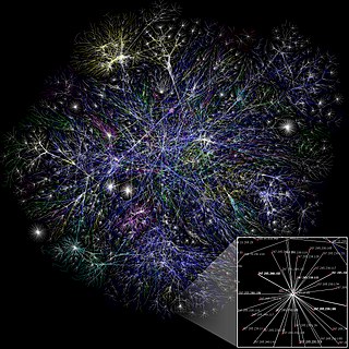
In graph theory, a random geometric graph (RGG) is the mathematically simplest spatial network, namely an undirected graph constructed by randomly placing N nodes in some metric space and connecting two nodes by a link if and only if their distance is in a given range, e.g. smaller than a certain neighborhood radius, r.

Sedimentation potential occurs when dispersed particles move under the influence of either gravity or centrifugation or electricity in a medium. This motion disrupts the equilibrium symmetry of the particle's double layer. While the particle moves, the ions in the electric double layer lag behind due to the liquid flow. This causes a slight displacement between the surface charge and the electric charge of the diffuse layer. As a result, the moving particle creates a dipole moment. The sum of all of the dipoles generates an electric field which is called sedimentation potential. It can be measured with an open electrical circuit, which is also called sedimentation current.

In fluid dynamics, the Burgers vortex or Burgers–Rott vortex is an exact solution to the Navier–Stokes equations governing viscous flow, named after Jan Burgers and Nicholas Rott. The Burgers vortex describes a stationary, self-similar flow. An inward, radial flow, tends to concentrate vorticity in a narrow column around the symmetry axis, while an axial stretching causes the vorticity to increase. At the same time, viscous diffusion tends to spread the vorticity. The stationary Burgers vortex arises when the three effects are in balance.

Mean-field particle methods are a broad class of interacting type Monte Carlo algorithms for simulating from a sequence of probability distributions satisfying a nonlinear evolution equation. These flows of probability measures can always be interpreted as the distributions of the random states of a Markov process whose transition probabilities depends on the distributions of the current random states. A natural way to simulate these sophisticated nonlinear Markov processes is to sample a large number of copies of the process, replacing in the evolution equation the unknown distributions of the random states by the sampled empirical measures. In contrast with traditional Monte Carlo and Markov chain Monte Carlo methods these mean-field particle techniques rely on sequential interacting samples. The terminology mean-field reflects the fact that each of the samples interacts with the empirical measures of the process. When the size of the system tends to infinity, these random empirical measures converge to the deterministic distribution of the random states of the nonlinear Markov chain, so that the statistical interaction between particles vanishes. In other words, starting with a chaotic configuration based on independent copies of initial state of the nonlinear Markov chain model, the chaos propagates at any time horizon as the size the system tends to infinity; that is, finite blocks of particles reduces to independent copies of the nonlinear Markov process. This result is called the propagation of chaos property. The terminology "propagation of chaos" originated with the work of Mark Kac in 1976 on a colliding mean-field kinetic gas model.

The Kubelka-Munk theory, devised by Paul Kubelka and Franz Munk, is a fundamental approach to modelling the appearance of paint films. As published in 1931, the theory addresses "the question of how the color of a substrate is changed by the application of a coat of paint of specified composition and thickness, and especially the thickness of paint needed to obscure the substrate". The mathematical relationship involves just two paint-dependent constants.

References

  1. Dahm, Donald J.; Dahm, Kevin D. (1999-06-01). "Representative Layer Theory for Diffuse Reflectance". Applied Spectroscopy. 53 (6): 647–654. Bibcode:1999ApSpe..53..647D. doi:10.1366/0003702991947298. ISSN   0003-7028. S2CID   96885077.
  2. 1 2 Dahm, Donald J.; Dahm, Kevin D.; Norris, Karl H. (2000-06-01). "Test of the Representative Layer Theory of Diffuse Reflectance Using Plane Parallel Samples". Journal of Near Infrared Spectroscopy. 8 (3): 171–181. Bibcode:2000JNIS....8..171D. doi:10.1255/jnirs.276. ISSN   0967-0335. S2CID   95860576.
  3. Bohren, Craig F.; Huffman, Donald R. (1998-04-23). Absorption and Scattering of Light by Small Particles (1 ed.). Wiley. doi:10.1002/9783527618156. ISBN   978-0-471-29340-8.
  4. Dahm, Kevin D.; Dahm, Donald J. (2004-06-01). "Relation of Representative Layer Theory to other Theories of Diffuse Reflection". Journal of Near Infrared Spectroscopy. 12 (3): 189–198. Bibcode:2004JNIS...12..189D. doi:10.1255/jnirs.426. ISSN   0967-0335. S2CID   123460305.
  5. "IV. On the intensity of the light reflected from or transmitted through a pile of plates". Proceedings of the Royal Society of London. 11: 545–556. 1862-12-31. doi: 10.1098/rspl.1860.0119 . ISSN   0370-1662.
  6. Strutt, John William (2009). Scientific Papers. Cambridge: Cambridge University Press. doi:10.1017/cbo9780511703966.009. ISBN   978-0-511-70396-6.
  7. Mie, Gustav (1908). "Beiträge zur Optik trüber Medien, speziell kolloidaler Metallösungen". Annalen der Physik. 330 (3): 377–445. Bibcode:1908AnP...330..377M. doi: 10.1002/andp.19083300302 . ISSN   1521-3889.
  8. Schuster, Arthur (January 1905). "Radiation Through a Foggy Atmosphere". The Astrophysical Journal. 21: 1. Bibcode:1905ApJ....21....1S. doi: 10.1086/141186 . ISSN   0004-637X.
  9. Kortüm, Gustav (1969). Reflectance spectroscopy Principles, methods, applications. Berlin: Springer. ISBN   978-3-642-88071-1. OCLC   714802320.
  10. Wendlandt, Wesley Wm; Hechtt, Harry (1966). Reflectance Spectroscopy (Chemical Analysis: A Series of Monographs on Analytical Chemistry and Its Applications, Volume 21). New York: Interscience Publishers. pp. 72–76.
  11. Williams, Phil (December 2019). "Karl H. Norris, the Father of Near-Infrared Spectroscopy". NIR News. 30 (7–8): 25–27. doi: 10.1177/0960336019875883 . ISSN   0960-3360.
  12. Hindle, Peter H (2021). Chap 1: Handbook of near-infrared analysis. Emil W. Ciurczak, Benoĭt Igne, Jerry Workman, Donald A. Burns (4 ed.). Boca Raton. ISBN   978-1-351-26988-9. OCLC   1200834251.{{cite book}}: CS1 maint: location missing publisher (link)
  13. Norris, Karl H. (December 2005). "Why Log(1/ R ) for Composition Analysis with Nir?". NIR News. 16 (8): 10–13. doi:10.1255/nirn.865. ISSN   0960-3360. S2CID   100866871.
  14. Dahm, Donald J. (2003-10-01). "An Intuitive Model of Diffuse Reflectance (and Infinitely Thick Samples)". NIR News. 14 (5): 5–6. doi:10.1255/nirn.731. ISSN   0960-3360. S2CID   97884223.
  15. 1 2 Hecht, Harry H (1976). "The Interpretation of Diffuse Reflectance Spectra". Journal of Research of the National Bureau of Standards Section A. 80A (4): 567–583. doi:10.6028/jres.080A.056. PMC   5293523 . PMID   32196278.
  16. Birth, Gerald R; Hecht, Harry G (1987). Chap 1: Physics of Near-InfraRed Reflectance in Near-infrared technology in the agricultural and food industries. American Association of Cereal Chemists.
  17. Dahm, Donald J.; Dahm, Kevin D. (1999-01-01). "Bridging the Continuum–Discontinuum Gap in the Theory of Diffuse Reflectance". Journal of Near Infrared Spectroscopy. 7 (1): 47–53. Bibcode:1999JNIS....7...47D. doi:10.1255/jnirs.233. ISSN   0967-0335. S2CID   96543562.
  18. Bodó, Zalán (1951). "Some optical properties of luminescent powders". Acta Physica Academiae Scientiarum Hungaricae. 1 (2): 135–150. Bibcode:1951AcPhy...1..135B. doi:10.1007/bf03156624. ISSN   0001-6705. S2CID   119987760.
  19. Benford, Frank (1946). "Radiation in a Diffusing Medium". Journal of the Optical Society of America. 36 (9): 524–554. doi:10.1364/JOSA.36.000524. PMID   21002043.
  20. Kubelka, Paul (1954-04-01). "New Contributions to the Optics of Intensely Light-Scattering Materials. Part II: Nonhomogeneous Layers*". JOSA. 44 (4): 330–335. doi:10.1364/JOSA.44.000330.
  21. Dahm, Donald J. (2007). Interpreting diffuse reflectance and transmittance : a theoretical introduction to absorption spectroscopy of scattering materials. Kevin D. Dahm. Chichester: NIR. p. 92. ISBN   978-1-901019-05-6. OCLC   132322356.
  22. IUPAC , Compendium of Chemical Terminology , 2nd ed. (the "Gold Book") (1997). Online corrected version: (2006) " decadic absorbance ". doi : 10.1351/goldbook.D01536
  23. Bertie, John E. (2006-08-15), Chalmers, John M.; Griffiths, Peter R. (eds.), "Glossary of Terms used in Vibrational Spectroscopy", Handbook of Vibrational Spectroscopy, Chichester, UK: John Wiley & Sons, Ltd, pp. s8401, doi:10.1002/0470027320.s8401, ISBN   978-0-471-98847-2 , retrieved 2021-05-25
  24. Dahm, Donald; Dahm, Kevin (2007-06-01). Interpreting Diffuse Reflectance and Transmittance: A Theoretical Introduction to Absorption Spectroscopy of Scattering Materials. IM Publications. doi:10.1255/978-1-901019-05-6. ISBN   978-1-901019-05-6.
  25. Dahm, Donald J. (2007). Interpreting diffuse reflectance and transmittance : a theoretical introduction to absorption spectroscopy of scattering materials. Kevin D. Dahm. Chichester: NIR. pp. 5–6. ISBN   978-1-901019-05-6. OCLC   132322356.
  26. Dahm, Kevin; Dahm, Donald (2021). Chap 4 in Handbook of near-infrared analysis. Emil W. Ciurczak, Benoĭt Igne, Jerry Workman, Donald A. Burns (4 ed.). Boca Raton: CRC Press. ISBN   978-1-351-26988-9. OCLC   1200834251.