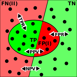
Statistical measures of the performance of a binary classification test
Sensitivity and specificity - The left half of the image with the solid dots represents individuals who have the condition, while the right half of the image with the hollow dots represents individuals who do not have the condition. The circle represents all individuals who tested positive.
In medicine and statistics, sensitivity and specificity mathematically describe the accuracy of a test that reports the presence or absence of a medical condition. If individuals who have the condition are considered "positive" and those who do not are considered "negative", then sensitivity is a measure of how well a test can identify true positives and specificity is a measure of how well a test can identify true negatives:
Sensitivity (true positive rate) is the probability of a positive test result, conditioned on the individual truly being positive.
Specificity (true negative rate) is the probability of a negative test result, conditioned on the individual truly being negative.
If the true status of the condition cannot be known, sensitivity and specificity can be defined relative to a "gold standard test" which is assumed correct. For all testing, both diagnoses and screening, there is usually a trade-off between sensitivity and specificity, such that higher sensitivities will mean lower specificities and vice versa.
A test which reliably detects the presence of a condition, resulting in a high number of true positives and low number of false negatives, will have a high sensitivity. This is especially important when the consequence of failing to treat the condition is serious and/or the treatment is very effective and has minimal side effects.
A test which reliably excludes individuals who do not have the condition, resulting in a high number of true negatives and low number of false positives, will have a high specificity. This is especially important when people who are identified as having a condition may be subjected to more testing, expense, stigma, anxiety, etc.
Sensitivity and specificity
The terms "sensitivity" and "specificity" were introduced by American biostatistician Jacob Yerushalmy in 1947.[1]
There are different definitions within laboratory quality control, wherein "analytical sensitivity" is defined as the smallest amount of substance in a sample that can accurately be measured by an assay (synonymously to detection limit), and "analytical specificity" is defined as the ability of an assay to measure one particular organism or substance, rather than others.[2] However, this article deals with diagnostic sensitivity and specificity as defined at top.
Application to screening study
Imagine a study evaluating a test that screens people for a disease. Each person taking the test either has or does not have the disease. The test outcome can be positive (classifying the person as having the disease) or negative (classifying the person as not having the disease). The test results for each subject may or may not match the subject's actual status. In that setting:
True positive: Sick people correctly identified as sick
False positive: Healthy people incorrectly identified as sick
True negative: Healthy people correctly identified as healthy
False negative: Sick people incorrectly identified as healthy
After getting the numbers of true positives, false positives, true negatives, and false negatives, the sensitivity and specificity for the test can be calculated. If it turns out that the sensitivity is high then any person who has the disease is likely to be classified as positive by the test. On the other hand, if the specificity is high, any person who does not have the disease is likely to be classified as negative by the test. An NIH web site has a discussion of how these ratios are calculated.[3]
Definition
Sensitivity
Consider the example of a medical test for diagnosing a condition. Sensitivity (sometimes also named the detection rate in a clinical setting) refers to the test's ability to correctly detect ill patients out of those who do have the condition.[4] Mathematically, this can be expressed as:
A negative result in a test with high sensitivity can be useful for "ruling out" disease,[4] since it rarely misdiagnoses those who do have the disease. A test with 100% sensitivity will recognize all patients with the disease by testing positive. In this case, a negative test result would definitively rule out the presence of the disease in a patient. However, a positive result in a test with high sensitivity is not necessarily useful for "ruling in" disease. Suppose a 'bogus' test kit is designed to always give a positive reading. When used on diseased patients, all patients test positive, giving the test 100% sensitivity. However, sensitivity does not take into account false positives. The bogus test also returns positive on all healthy patients, giving it a false positive rate of 100%, rendering it useless for detecting or "ruling in" the disease.[citation needed]
The calculation of sensitivity does not take into account indeterminate test results. If a test cannot be repeated, indeterminate samples either should be excluded from the analysis (the number of exclusions should be stated when quoting sensitivity) or can be treated as false negatives (which gives the worst-case value for sensitivity and may therefore underestimate it).[citation needed]
A test with a higher sensitivity has a lower type II error rate.
Specificity
Consider the example of a medical test for diagnosing a disease. Specificity refers to the test's ability to correctly reject healthy patients without a condition. Mathematically, this can be written as:
A positive result in a test with high specificity can be useful for "ruling in" disease, since the test rarely gives positive results in healthy patients.[5] A test with 100% specificity will recognize all patients without the disease by testing negative, so a positive test result would definitively rule in the presence of the disease. However, a negative result from a test with high specificity is not necessarily useful for "ruling out" disease. For example, a test that always returns a negative test result will have a specificity of 100% because specificity does not consider false negatives. A test like that would return negative for patients with the disease, making it useless for "ruling out" the disease.
A test with a higher specificity has a lower type I error rate.
Graphical illustration
High sensitivity and low specificity
Low sensitivity and high specificity
A graphical illustration of sensitivity and specificity
The above graphical illustration is meant to show the relationship between sensitivity and specificity. The black, dotted line in the center of the graph is where the sensitivity and specificity are the same. As one moves to the left of the black dotted line, the sensitivity increases, reaching its maximum value of 100% at line A, and the specificity decreases. The sensitivity at line A is 100% because at that point there are zero false negatives, meaning that all the negative test results are true negatives. When moving to the right, the opposite applies, the specificity increases until it reaches the B line and becomes 100% and the sensitivity decreases. The specificity at line B is 100% because the number of false positives is zero at that line, meaning all the positive test results are true positives.
The middle solid line in both figures that show the level of sensitivity and specificity is the test cutoff point. As previously described, moving this line results in a trade-off between the level of sensitivity and specificity. The left-hand side of this line contains the data points that tests below the cut off point and are considered negative (the blue dots indicate the False Negatives (FN), the white dots True Negatives (TN)). The right-hand side of the line shows the data points that tests above the cut off point and are considered positive (red dots indicate False Positives (FP)). Each side contains 40 data points.
For the figure that shows high sensitivity and low specificity, there are 3 FN and 8 FP. Using the fact that positive results = true positives (TP) + FP, we get TP = positive results - FP, or TP = 40 - 8 = 32. The number of sick people in the data set is equal to TP + FN, or 32 + 3 = 35. The sensitivity is therefore 32 / 35 = 91.4%. Using the same method, we get TN = 40 - 3 = 37, and the number of healthy people 37 + 8 = 45, which results in a specificity of 37 / 45 = 82.2%.
For the figure that shows low sensitivity and high specificity, there are 8 FN and 3 FP. Using the same method as the previous figure, we get TP = 40 - 3 = 37. The number of sick people is 37 + 8 = 45, which gives a sensitivity of 37 / 45 = 82.2%. There are 40 - 8 = 32 TN. The specificity therefore comes out to 32 / 35 = 91.4%.
A test result with 100 percent sensitivity
A test result with 100 percent specificity
The red dot indicates the patient with the medical condition. The red background indicates the area where the test predicts the data point to be positive. The true positive in this figure is 6, and false negatives of 0 (because all positive condition is correctly predicted as positive). Therefore, the sensitivity is 100% (from 6 / (6 + 0)). This situation is also illustrated in the previous figure where the dotted line is at position A (the left-hand side is predicted as negative by the model, the right-hand side is predicted as positive by the model). When the dotted line, test cut-off line, is at position A, the test correctly predicts all the population of the true positive class, but it will fail to correctly identify the data point from the true negative class.
Similar to the previously explained figure, the red dot indicates the patient with the medical condition. However, in this case, the green background indicates that the test predicts that all patients are free of the medical condition. The number of data point that is true negative is then 26, and the number of false positives is 0. This result in 100% specificity (from 26 / (26 + 0)). Therefore, sensitivity or specificity alone cannot be used to measure the performance of the test.
Medical usage
In medical diagnosis, test sensitivity is the ability of a test to correctly identify those with the disease (true positive rate), whereas test specificity is the ability of the test to correctly identify those without the disease (true negative rate). If 100 patients known to have a disease were tested, and 43 test positive, then the test has 43% sensitivity. If 100 with no disease are tested and 96 return a completely negative result, then the test has 96% specificity. Sensitivity and specificity are prevalence-independent test characteristics, as their values are intrinsic to the test and do not depend on the disease prevalence in the population of interest.[6]Positive and negative predictive values, but not sensitivity or specificity, are values influenced by the prevalence of disease in the population that is being tested. These concepts are illustrated graphically in this applet Bayesian clinical diagnostic model which show the positive and negative predictive values as a function of the prevalence, sensitivity and specificity.
Misconceptions
It is often claimed that a highly specific test is effective at ruling in a disease when positive, while a highly sensitive test is deemed effective at ruling out a disease when negative.[7][8] This has led to the widely used mnemonics SPPIN and SNNOUT, according to which a highly specific test, when positive, rules in disease (SP-P-IN), and a highly sensitive test, when negative, rules out disease (SN-N-OUT). Both rules of thumb are, however, inferentially misleading, as the diagnostic power of any test is determined by the prevalence of the condition being tested, the test's sensitivity and its specificity.[9][10][11] The SNNOUT mnemonic has some validity when the prevalence of the condition in question is extremely low in the tested sample.
The tradeoff between specificity and sensitivity is explored in ROC analysis as a trade off between TPR and FPR (that is, recall and fallout).[12] Giving them equal weight optimizes informedness = specificity + sensitivity − 1 = TPR − FPR, the magnitude of which gives the probability of an informed decision between the two classes (>0 represents appropriate use of information, 0 represents chance-level performance, <0 represents perverse use of information).[13]
Sensitivity index
The sensitivity index or d′ (pronounced "dee-prime") is a statistic used in signal detection theory. It provides the separation between the means of the signal and the noise distributions, compared against the standard deviation of the noise distribution. For normally distributed signal and noise with mean and standard deviations and , and and , respectively, d′ is defined as:
The relationship between sensitivity, specificity, and similar terms can be understood using the following table. Consider a group with P positive instances and N negative instances of some condition. The four outcomes can be formulated in a 2×2 contingency table or confusion matrix, as well as derivations of several metrics using the four outcomes, as follows:
This hypothetical screening test (fecal occult blood test) correctly identified two-thirds (66.7%) of patients with colorectal cancer.[lower-alpha 1] Unfortunately, factoring in prevalence rates reveals that this hypothetical test has a high false positive rate, and it does not reliably identify colorectal cancer in the overall population of asymptomatic people (PPV=10%).
On the other hand, this hypothetical test demonstrates very accurate detection of cancer-free individuals (NPV≈99.5%). Therefore, when used for routine colorectal cancer screening with asymptomatic adults, a negative result supplies important data for the patient and doctor, such as ruling out cancer as the cause of gastrointestinal symptoms or reassuring patients worried about developing colorectal cancer.
Estimation of errors in quoted sensitivity or specificity
Sensitivity and specificity values alone may be highly misleading. The 'worst-case' sensitivity or specificity must be calculated in order to avoid reliance on experiments with few results. For example, a particular test may easily show 100% sensitivity if tested against the gold standard four times, but a single additional test against the gold standard that gave a poor result would imply a sensitivity of only 80%. A common way to do this is to state the binomial proportion confidence interval, often calculated using a Wilson score interval.
Confidence intervals for sensitivity and specificity can be calculated, giving the range of values within which the correct value lies at a given confidence level (e.g., 95%).[26]
Terminology in information retrieval
In information retrieval, the positive predictive value is called precision, and sensitivity is called recall. Unlike the Specificity vs Sensitivity tradeoff, these measures are both independent of the number of true negatives, which is generally unknown and much larger than the actual numbers of relevant and retrieved documents. This assumption of very large numbers of true negatives versus positives is rare in other applications.[13]
The F-score can be used as a single measure of performance of the test for the positive class. The F-score is the harmonic mean of precision and recall:
In the traditional language of statistical hypothesis testing, the sensitivity of a test is called the statistical power of the test, although the word power in that context has a more general usage that is not applicable in the present context. A sensitive test will have fewer Type II errors.
Terminology in genome analysis
Similarly to the domain of information retrieval, in the research area of gene prediction, the number of true negatives (non-genes) in genomic sequences is generally unknown and much larger than the actual number of genes (true positives). The convenient and intuitively understood term specificity in this research area has been frequently used with the mathematical formula for precision and recall as defined in biostatistics. The pair of thus defined specificity (as positive predictive value) and sensitivity (true positive rate) represent major parameters characterizing the accuracy of gene prediction algorithms. [27][28][29][30] Conversely, the term specificity in a sense of true negative rate would have little, if any, application in the genome analysis research area.
↑ There are advantages and disadvantages for all medical screening tests. Clinical practice guidelines, such as those for colorectal cancer screening, describe these risks and benefits.[24][25]
Related Research Articles
In epidemiology, prevalence is the proportion of a particular population found to be affected by a medical condition at a specific time. It is derived by comparing the number of people found to have the condition with the total number of people studied and is usually expressed as a fraction, a percentage, or the number of cases per 10,000 or 100,000 people. Prevalence is most often used in questionnaire studies.
Binary classification is the task of classifying the elements of a set into one of two groups on the basis of a classification rule. Typical binary classification problems include:
HIV tests are used to detect the presence of the human immunodeficiency virus (HIV), the virus that causes acquired immunodeficiency syndrome (AIDS), in serum, saliva, or urine. Such tests may detect antibodies, antigens, or RNA.
In medicine and medical statistics, the gold standard, criterion standard, or reference standard is the diagnostic test or benchmark that is the best available under reasonable conditions. It is the test against which new tests are compared to gauge their validity, and it is used to evaluate the efficacy of treatments.
In the field of machine learning and specifically the problem of statistical classification, a confusion matrix, also known as error matrix, is a specific table layout that allows visualization of the performance of an algorithm, typically a supervised learning one; in unsupervised learning it is usually called a matching matrix.
A receiver operating characteristic curve, or ROC curve, is a graphical plot that illustrates the performance of a binary classifier model at varying threshold values.
In evidence-based medicine, likelihood ratios are used for assessing the value of performing a diagnostic test. They use the sensitivity and specificity of the test to determine whether a test result usefully changes the probability that a condition exists. The first description of the use of likelihood ratios for decision rules was made at a symposium on information theory in 1954. In medicine, likelihood ratios were introduced between 1975 and 1980.
D-dimer is a dimer that is a fibrin degradation product, a small protein fragment present in the blood after a blood clot is degraded by fibrinolysis. It is so named because it contains two D fragments of the fibrin protein joined by a cross-link, hence forming a protein dimer.
Pathognomonic is a term, often used in medicine, that means "characteristic for a particular disease". A pathognomonic sign is a particular sign whose presence means that a particular disease is present beyond any doubt. Labelling a sign or symptom "pathognomonic" represents a marked intensification of a "diagnostic" sign or symptom.
The positive and negative predictive values are the proportions of positive and negative results in statistics and diagnostic tests that are true positive and true negative results, respectively. The PPV and NPV describe the performance of a diagnostic test or other statistical measure. A high result can be interpreted as indicating the accuracy of such a statistic. The PPV and NPV are not intrinsic to the test ; they depend also on the prevalence. Both PPV and NPV can be derived using Bayes' theorem.
Given a population whose members each belong to one of a number of different sets or classes, a classification rule or classifier is a procedure by which the elements of the population set are each predicted to belong to one of the classes. A perfect classification is one for which every element in the population is assigned to the class it really belongs to. The bayes classifier is the classifier which assigns classes optimally based on the known attributes of the elements to be classified.
A medical test is a medical procedure performed to detect, diagnose, or monitor diseases, disease processes, susceptibility, or to determine a course of treatment. Medical tests such as, physical and visual exams, diagnostic imaging, genetic testing, chemical and cellular analysis, relating to clinical chemistry and molecular diagnostics, are typically performed in a medical setting.
Youden's J statistic is a single statistic that captures the performance of a dichotomous diagnostic test. (Bookmaker) Informedness is its generalization to the multiclass case and estimates the probability of an informed decision.
In pattern recognition, information retrieval, object detection and classification, precision and recall are performance metrics that apply to data retrieved from a collection, corpus or sample space.
Pre-test probability and post-test probability are the probabilities of the presence of a condition before and after a diagnostic test, respectively. Post-test probability, in turn, can be positive or negative, depending on whether the test falls out as a positive test or a negative test, respectively. In some cases, it is used for the probability of developing the condition of interest in the future.
In medical testing with binary classification, the diagnostic odds ratio (DOR) is a measure of the effectiveness of a diagnostic test. It is defined as the ratio of the odds of the test being positive if the subject has a disease relative to the odds of the test being positive if the subject does not have the disease.
Receiver Operating Characteristic Curve Explorer and Tester (ROCCET) is an open-access web server for performing biomarker analysis using ROC curve analyses on metabolomic data sets. ROCCET is designed specifically for performing and assessing a standard binary classification test. ROCCET accepts metabolite data tables, with or without clinical/observational variables, as input and performs extensive biomarker analysis and biomarker identification using these input data. It operates through a menu-based navigation system that allows users to identify or assess those clinical variables and/or metabolites that contain the maximal diagnostic or class-predictive information. ROCCET supports both manual and semi-automated feature selection and is able to automatically generate a variety of mathematical models that maximize the sensitivity and specificity of the biomarker(s) while minimizing the number of biomarkers used in the biomarker model. ROCCET also supports the rigorous assessment of the quality and robustness of newly discovered biomarkers using permutation testing, hold-out testing and cross-validation.
The evaluation of binary classifiers compares two methods of assigning a binary attribute, one of which is usually a standard method and the other is being investigated. There are many metrics that can be used to measure the performance of a classifier or predictor; different fields have different preferences for specific metrics due to different goals. For example, in medicine sensitivity and specificity are often used, while in computer science precision and recall are preferred. An important distinction is between metrics that are independent on the prevalence, and metrics that depend on the prevalence – both types are useful, but they have very different properties.
A false positive is an error in binary classification in which a test result incorrectly indicates the presence of a condition, while a false negative is the opposite error, where the test result incorrectly indicates the absence of a condition when it is actually present. These are the two kinds of errors in a binary test, in contrast to the two kinds of correct result. They are also known in medicine as a false positivediagnosis, and in statistical classification as a false positiveerror.
The discipline of forensic epidemiology (FE) is a hybrid of principles and practices common to both forensic medicine and epidemiology. FE is directed at filling the gap between clinical judgment and epidemiologic data for determinations of causality in civil lawsuits and criminal prosecution and defense.
References
↑ Yerushalmy J (1947). "Statistical problems in assessing methods of medical diagnosis with special reference to x-ray techniques". Public Health Reports. 62 (2): 1432–39. doi:10.2307/4586294. JSTOR4586294. PMID20340527. S2CID19967899.
↑ Boyko EJ (Apr–Jun 1994). "Ruling out or ruling in disease with the most sensitive or specific diagnostic test: short cut or wrong turn?". Medical Decision Making. 14 (2): 175–9. doi:10.1177/0272989X9401400210. PMID8028470. S2CID31400167.
↑ Brooks H, Brown B, Ebert B, Ferro C, Jolliffe I, Koh TY, Roebber P, Stephenson D (2015-01-26). "WWRP/WGNE Joint Working Group on Forecast Verification Research". Collaboration for Australian Weather and Climate Research. World Meteorological Organisation. Retrieved 2019-07-17.
↑ Lin JS, Piper MA, Perdue LA, Rutter CM, Webber EM, O'Connor E, Smith N, Whitlock EP (21 June 2016). "Screening for Colorectal Cancer". JAMA. 315 (23): 2576–2594. doi:10.1001/jama.2016.3332. ISSN0098-7484. PMID27305422.
This page is based on this Wikipedia article Text is available under the CC BY-SA 4.0 license; additional terms may apply. Images, videos and audio are available under their respective licenses.