Thomson problem

Last updated

The objective of the Thomson problem is to determine the minimum electrostatic potential energy configuration of N electrons constrained to the surface of a unit sphere that repel each other with a force given by Coulomb's law. The physicist J. J. Thomson posed the problem in 1904 [1] after proposing an atomic model, later called the plum pudding model, based on his knowledge of the existence of negatively charged electrons within neutrally-charged atoms.

Contents

Related problems include the study of the geometry of the minimum energy configuration and the study of the large N behavior of the minimum energy.

Mathematical statement

The electrostatic interaction energy occurring between each pair of electrons of equal charges (, with the elementary charge of an electron) is given by Coulomb's law,

where is the electric constant and is the distance between each pair of electrons located at points on the sphere defined by vectors and , respectively.

Simplified units of and (the Coulomb constant) are used without loss of generality. Then,

The total electrostatic potential energy of each N-electron configuration may then be expressed as the sum of all pair-wise interaction energies

The global minimization of over all possible configurations of N distinct points is typically found by numerical minimization algorithms.

Thomson's problem is related to the 7th of the eighteen unsolved mathematics problems proposed by the mathematician Steve Smale — "Distribution of points on the 2-sphere". [2] The main difference is that in Smale's problem the function to minimise is not the electrostatic potential but a logarithmic potential given by A second difference is that Smale's question is about the asymptotic behaviour of the total potential when the number N of points goes to infinity, not for concrete values of N.

Example

The solution of the Thomson problem for two electrons is obtained when both electrons are as far apart as possible on opposite sides of the origin, , or

Known exact solutions

Schematic geometric solutions of the mathematical Thomson Problem for up to N = 5 electrons. N 2 to 5 ThomsonSolutions.png
Schematic geometric solutions of the mathematical Thomson Problem for up to N = 5 electrons.

Mathematically exact minimum energy configurations have been rigorously identified in only a handful of cases.

Geometric solutions of the Thomson problem for N = 4, 6, and 12 electrons are Platonic solids whose faces are all congruent equilateral triangles. Numerical solutions for N = 8 and 20 are not the regular convex polyhedral configurations of the remaining two Platonic solids, the cube and dodecahedron respectively. [7]

Generalizations

One can also ask for ground states of particles interacting with arbitrary potentials. To be mathematically precise, let f be a decreasing real-valued function, and define the energy functional

Traditionally, one considers also known as Riesz -kernels. For integrable Riesz kernels see the 1972 work of Landkof. [8] For non-integrable Riesz kernels, the Poppy-seed bagel theorem holds, see the 2004 work of Hardin and Saff. [9] Notable cases include: [10]

One may also consider configurations of N points on a sphere of higher dimension. See spherical design.

Solution algorithms

Several algorithms have been applied to this problem. The focus since the millennium has been on local optimization methods applied to the energy function, although random walks have made their appearance: [10]

While the objective is to minimize the global electrostatic potential energy of each N-electron case, several algorithmic starting cases are of interest.

Continuous spherical shell charge

The extreme upper energy limit of the Thomson Problem is given by
N
2
/
2
{\displaystyle N^{2}/2}
for a continuous shell charge followed by N(N - 1)/2, the energy associated with a random distribution of N electrons. Significantly lower energy of a given N-electron solution of the Thomson Problem with one charge at its origin is readily obtained by
U
(
N
)
+
N
{\displaystyle U(N)+N}
, where
U
(
N
)
{\displaystyle U(N)}
are solutions of the Thomson Problem. ThomsonProblem Related Energies LaFave.png
The extreme upper energy limit of the Thomson Problem is given by for a continuous shell charge followed by N(N − 1)/2, the energy associated with a random distribution of N electrons. Significantly lower energy of a given N-electron solution of the Thomson Problem with one charge at its origin is readily obtained by , where are solutions of the Thomson Problem.

The energy of a continuous spherical shell of charge distributed across its surface is given by

and is, in general, greater than the energy of every Thomson problem solution. Note: Here N is used as a continuous variable that represents the infinitely divisible charge, Q, distributed across the spherical shell. For example, a spherical shell of represents the uniform distribution of a single electron's charge, , across the entire shell.

Randomly distributed point charges

The global energy of a system of electrons distributed in a purely random manner across the surface of the sphere is given by

and is, in general, greater than the energy of every Thomson problem solution.

Here, N is a discrete variable that counts the number of electrons in the system. As well, .

Charge-centered distribution

For every Nth solution of the Thomson problem there is an th configuration that includes an electron at the origin of the sphere whose energy is simply the addition of N to the energy of the Nth solution. That is, [11]

Thus, if is known exactly, then is known exactly.

In general, is greater than , but is remarkably closer to each th Thomson solution than and . Therefore, the charge-centered distribution represents a smaller "energy gap" to cross to arrive at a solution of each Thomson problem than algorithms that begin with the other two charge configurations.

Relations to other scientific problems

The Thomson problem is a natural consequence of J. J. Thomson's plum pudding model in the absence of its uniform positive background charge. [12]

"No fact discovered about the atom can be trivial, nor fail to accelerate the progress of physical science, for the greater part of natural philosophy is the outcome of the structure and mechanism of the atom."

—Sir J. J. Thomson [13]

Though experimental evidence led to the abandonment of Thomson's plum pudding model as a complete atomic model, irregularities observed in numerical energy solutions of the Thomson problem have been found to correspond with electron shell-filling in naturally occurring atoms throughout the periodic table of elements. [14]

The Thomson problem also plays a role in the study of other physical models including multi-electron bubbles and the surface ordering of liquid metal drops confined in Paul traps.

The generalized Thomson problem arises, for example, in determining arrangements of protein subunits that comprise the shells of spherical viruses. The "particles" in this application are clusters of protein subunits arranged on a shell. Other realizations include regular arrangements of colloid particles in colloidosomes, proposed for encapsulation of active ingredients such as drugs, nutrients or living cells, fullerene patterns of carbon atoms, and VSEPR theory. An example with long-range logarithmic interactions is provided by Abrikosov vortices that form at low temperatures in a superconducting metal shell with a large monopole at its center.

Configurations of smallest known energy

In the following table[ citation needed ] is the number of points (charges) in a configuration, is the energy, the symmetry type is given in Schönflies notation (see Point groups in three dimensions), and are the positions of the charges. Most symmetry types require the vector sum of the positions (and thus the electric dipole moment) to be zero.

It is customary to also consider the polyhedron formed by the convex hull of the points. Thus, is the number of vertices where the given number of edges meet, is the total number of edges, is the number of triangular faces, is the number of quadrilateral faces, and is the smallest angle subtended by vectors associated with the nearest charge pair. Note that the edge lengths are generally not equal. Thus, except in the cases N = 2, 3, 4, 6, 12, and the geodesic polyhedra, the convex hull is only topologically equivalent to the figure listed in the last column. [15]

N Symmetry Equivalent polyhedron
20.50000000002180.000° digon
31.732050808032120.000° triangle
43.6742346140400000640109.471° tetrahedron
56.474691495023000096090.000° triangular dipyramid
69.9852813740060000128090.000° octahedron
714.45297741400520001510072.000° pentagonal dipyramid
819.6752878610080000168271.694° square antiprism
925.75998653100360002114069.190° triaugmented triangular prism
1032.71694946000280002416064.996° gyroelongated square dipyramid
1140.5964505100.0132196350281002718058.540° edge-contracted icosahedron
1249.165253058000120003020063.435° icosahedron
(geodesic sphere {3,5+}1,0)
1358.8532306120.00882036701102003322052.317°
1469.306363297000122003624052.866°gyroelongated hexagonal dipyramid
1580.670244114000123003926049.225°
1692.911655302000124004228048.936°
17106.050404829000125004530050.108°double-gyroelongated pentagonal dipyramid
18120.08446744700288004832047.534°
19135.0894675570.00013516300145005032144.910°
20150.881568334000128005436046.093°
21167.6416223990.001406124011010005738044.321°
22185.2875361490001210006040043.302°
23203.9301906630001211006342041.481°
24223.347074052000240006032642.065° snub cube
25243.8127602990.001021305001411006844139.610°
26265.1333263170.001919065001214007248038.842°
27287.3026150330001215007550039.940°
28310.4915423580001216007852037.824°
29334.6344399200001217008154036.391°
30359.6039459040001218008456036.942°
31385.5308380630.003204712001219008758036.373°
32412.2612746510001220009060037.377° pentakis dodecahedron
(geodesic sphere {3,5+}1,1)
33440.2040574480.004356481001517109260133.700°
34468.9048532810001222009664033.273°
35498.5698724910.000419208001223009966033.100°
36529.12240837500012240010268033.229°
37560.61888773100012250010570032.332°
38593.03850356600012260010872033.236°
39626.38900901700012270011174032.053°
40660.67527883500012280011476031.916°
41695.91674434200012290011778031.528°
42732.07810754400012300012080031.245°
43769.1908464590.0003996680012310012382030.867°
44807.17426308500024200012072631.258°
45846.18840106100012330012986030.207°
46886.16711363900012340013288029.790°
47927.0592706800.0024829140014330013488128.787°
48968.71345534400024240013280629.690°
491011.5571826540.0015293410012370014194028.387°
501055.18231472600012380014496029.231°
511099.81929031900012390014798028.165°
521145.4189643190.00045732700124000150100027.670°
531191.9222904160.0002784690018350015096327.137°
541239.3614747290.00013787000124200156104027.030°
551287.7727207830.00039169600124300159106026.615°
561337.094945276000124400162108026.683°
571387.383229253000124500165110026.702°
581438.618250640000124600168112026.155°
591490.7733352790.00015428600144320171114026.170°
601543.830400976000124800174116025.958°
611597.9418301990.00109171700124900177118025.392°
621652.909409898000125000180120025.880°
631708.879681503000125100183122025.257°
641765.802577927000125200186124024.920°
651823.6679602640.00039951500125300189126024.527°
661882.4415253040.00077624500125400192128024.765°
671942.122700406000125500195130024.727°
682002.874701749000125600198132024.433°
692064.533483235000125700201134024.137°
702127.100901551000125000200128424.291°
712190.6499064250.00125676900145520207138023.803°
722255.001190975000126000210140024.492° geodesic sphere {3,5+}2,1
732320.6338837450.00157295900126100213142022.810°
742387.0729818380.00064153900126200216144022.966°
752454.369689040000126300219146022.736°
762522.6748718410.00094347400126400222148022.886°
772591.850152354000126500225150023.286°
782662.046474566000126600228152023.426°
792733.2483574790.00070292100126310230152122.636°
802805.355875981000166400232152222.778°
812878.5228296640.00019428900126900237158021.892°
822952.569675286000127000240160022.206°
833027.5284889210.00033981500146720243162021.646°
843103.4651244310.00040197300127200246164021.513°
853180.3614429390.00041658100127300249166021.498°
863258.2116057130.00137893200127400252168021.522°
873337.0007500140.00075486300127500255170021.456°
883416.720196758000127600258172021.486°
893497.4390186250.00007089100127700261174021.182°
903579.091222723000127800264176021.230°
913661.7136993200.00003322100127900267178021.105°
923745.291636241000128000270180021.026°
933829.8443384210.00021324600128100273182020.751°
943915.309269620000128200276184020.952°
954001.7716755650.00011663800128300279186020.711°
964089.1540100600.00003631000128400282188020.687°
974177.5335996220.00009643700128500285190020.450°
984266.8224641560.00011291600128600288192020.422°
994357.1391631320.00015650800128700291194020.284°
1004448.350634331000128800294196020.297°
1014540.590051694000128900297198020.011°
1024633.736565899000129000300200020.040°
1034727.8366168330.00020124500129100303202019.907°
1044822.876522746000129200306204019.957°
1054919.000637616000129300309206019.842°
1065015.984595705000129400312208019.658°
1075113.9535477240.00006413700129500315210019.327°
1085212.8135078310.00043252500129600318212019.327°
1095312.7350799200.00064729900149320321214019.103°
1105413.549294192000129800324216019.476°
1115515.293214587000129900327218019.255°
1125618.0448823270001210000330220019.351°
1135721.8249780270001210100333222018.978°
1145826.5215721630.000149772001210200336224018.836°
1155932.1812857770.000049972001210300339226018.458°
1166038.8155935790.000259726001210400342228018.386°
1176146.3424465790.000127609001210500345230018.566°
1186254.8770277900.000332475001210600348232018.455°
1196364.3473174790.000685590001210700351234018.336°
1206474.7563249800.001373062001210800354236018.418°
1216586.1219495840.000838863001210900357238018.199°
1226698.3744992610001211000360240018.612° geodesic sphere {3,5+}2,2
1236811.8272281740.001939754001410720363242017.840°
1246926.1699741930001211200366244018.111°
1257041.4732640230.000088274001211300369246017.867°
1267157.6692248670021610080372248017.920°
1277274.8195046750001211500375250017.877°
1287393.0074430680.000054132001211600378252017.814°
1297512.1073192680.000030099001211700381254017.743°
1307632.1673789120.000025622001211800384256017.683°
1317753.2051669410.000305133001211900387258017.511°
1327875.0453427970001212000390260017.958° geodesic sphere {3,5+}3,1
1337998.1792128980.000591438001212100393262017.133°
1348122.0897211940.000470268001212200396264017.214°
1358246.9094869920001212300399266017.431°
1368372.7433025390001212400402268017.485°
1378499.5344947820001212500405270017.560°
1388627.4063898800.000473576001212600408272016.924°
1398756.2270560570.000404228001212700411274016.673°
1408885.9806090410.000630351001312610414276016.773°
1419016.6153491900.000376365001412601417278016.962°
1429148.2715799930.000550138001213000420280016.840°
1439280.8398511920.000255449001213100423282016.782°
1449414.3717944600001213200426284016.953°
1459548.9288372320.000094938001213300429286016.841°
1469684.3818255750001213400432288016.905°
1479820.9323783730.000636651001213500435290016.458°
1489958.4060042700.000203701001213600438292016.627°
14910096.8599073970.000638186001413320441294016.344°
15010236.1964367010001213800444296016.405°
15110376.5714692750.000153836001213900447298016.163°
15210517.8675928780001214000450300016.117°
15310660.0827482370001214100453302016.390°
15410803.3724211410.000735800001214200456304016.078°
15510947.5746922790.000603670001214300459306015.990°
15611092.7983114560.000508534001214400462308015.822°
15711238.9030411560.000357679001214500465310015.948°
15811385.9901861970.000921918001214600468312015.987°
15911534.0239609560.000381457001214700471314015.960°
16011683.0548055490001214800474316015.961°
16111833.0847394650.000056447001214900477318015.810°
16211984.0503358140001215000480320015.813°
16312136.0130532200.000120798001215100483322015.675°
16412288.9301053200001215200486324015.655°
16512442.8044513730.000091119001215300489326015.651°
16612597.6490713230001614640492328015.607°
16712753.4694297500.000097382001215500495330015.600°
16812910.2126722680001215600498332015.655°
16913068.0064511270.000068102001315510501334015.537°
17013226.6810785410001215800504336015.569°
17113386.3559307170001215900507338015.497°
17213547.0181087870.000547291001415620510340015.292°
17313708.6352430340.000286544001216100513342015.225°
17413871.1870922920001216200516344015.366°
17514034.7813069290.000026686001216300519346015.252°
17614199.3547756320.000283978001216400522348015.101°
17714364.8375452980001216500525350015.269°
17814531.3095525870001216600528352015.145°
17914698.7545942200.000125113001316510531354014.968°
18014867.0999275250001216800534356015.067°
18115036.4672397690.000304193001216900537358015.002°
18215206.7306109060001217000540360015.155°
18315378.1665710280.000467899001217100543362014.747°
18415550.4214503110001217200546364014.932°
18515723.7200740720.000389762001217300549366014.775°
18615897.8974370480.000389762001217400552368014.739°
18716072.9751863200001217500555370014.848°
18816249.2226788790001217600558372014.740°
18916426.3719388620.000020732001217700561374014.671°
19016604.4283385010.000586804001217800564376014.501°
19116783.4522193620.001129202001317710567378014.195°
19216963.3383864600001218000570380014.819° geodesic sphere {3,5+}3,2
19317144.5647408800.000985192001218100573382014.144°
19417326.6161364710.000322358001218200576384014.350°
19517509.4893039300001218300579386014.375°
19617693.4605480820.000315907001218400582388014.251°
19717878.3401625710001218500585390014.147°
19818064.2621771950.000011149001218600588392014.237°
19918251.0824956400.000534779001218700591394014.153°
20018438.8427175300001218800594396014.222°
20118627.5912262440.001048859001318710597398013.830°
20218817.2047182620001219000600400014.189°
20319007.9812045800.000600343001219100603402013.977°
20419199.5407756030001219200606404014.291°
21220768.0530859640001220000630420014.118° geodesic sphere {3,5+}4,1
21421169.9104103750001220200636424013.771°
21621575.5963778690001220400642428013.735°
21721779.8560804180001220500645430013.902°
23224961.2523189340001222000690460013.260°
25530264.4242512810001224300759506012.565°
25630506.6875158470001224400762508012.572°
25730749.9414173460001224500765510012.672°
27234515.1932926810001226000810540012.335° geodesic sphere {3,5+}3,3
28237147.2944184620001227000840560012.166° geodesic sphere {3,5+}4,2
29239877.0080129090001228000870580011.857°
30643862.5697807970001229400912608011.628°
31245629.3138040020.000306163001230000930620011.299°
31546525.8256434320001230300939626011.337°
31747128.3103445200001230500945630011.423°
31847431.0560200430001230600948632011.219°
33452407.7281278220001232200996664011.058°
34856967.47245433400012336001038692010.721°
35759999.92293959800012345001065710010.728°
35860341.83092458800012346001068712010.647°
37265230.02712255700012360001110740010.531° geodesic sphere {3,5+}4,3
38268839.42683921500012370001140760010.379°
39071797.03533595300012378001164776010.222°
39272546.25837088900012380001170780010.278°
40075582.44851221300012388001194796010.068°
40276351.19243267300012390001200800010.099°
43288353.70968195600024396120129086009.556°
44895115.54698620900024412120133889209.322°
460100351.76310867300024424120137491609.297°
468103920.87171512700024432120139893209.120°
470104822.88632427900024434120140493609.059°

According to a conjecture, if , p is the polyhedron formed by the convex hull of m points, q is the number of quadrilateral faces of p, then the solution for m electrons is f(m): . [16] [ clarification needed ]

Related Research Articles

<span class="mw-page-title-main">Atomic orbital</span> Function describing an electron in an atom

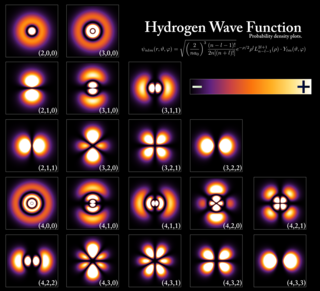
In quantum mechanics, an atomic orbital is a function describing the location and wave-like behavior of an electron in an atom. This function describes the electron's charge distribution around the atom's nucleus, and can be used to calculate the probability of finding an electron in a specific region around the nucleus.

<span class="mw-page-title-main">Pauli exclusion principle</span> Quantum mechanics rule: identical fermions cannot occupy the same quantum state simultaneously

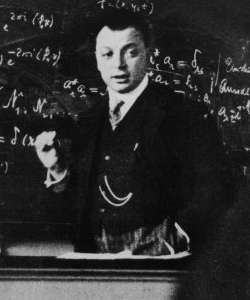
In quantum mechanics, the Pauli exclusion principle states that two or more identical particles with half-integer spins cannot simultaneously occupy the same quantum state within a system that obeys the laws of quantum mechanics. This principle was formulated by Austrian physicist Wolfgang Pauli in 1925 for electrons, and later extended to all fermions with his spin–statistics theorem of 1940.

The quantum Hall effect is a quantized version of the Hall effect which is observed in two-dimensional electron systems subjected to low temperatures and strong magnetic fields, in which the Hall resistance Rxy exhibits steps that take on the quantized values

<span class="mw-page-title-main">Capacitance</span> Ability of a body to store an electrical charge

Capacitance is the capability of a material object or device to store electric charge. It is measured by the charge in response to a difference in electric potential, expressed as the ratio of those quantities. Commonly recognized are two closely related notions of capacitance: self capacitance and mutual capacitance. An object that can be electrically charged exhibits self capacitance, for which the electric potential is measured between the object and ground. Mutual capacitance is measured between two components, and is particularly important in the operation of the capacitor, an elementary linear electronic component designed to add capacitance to an electric circuit.

<span class="mw-page-title-main">Packing problems</span> Problems which attempt to find the most efficient way to pack objects into containers

Packing problems are a class of optimization problems in mathematics that involve attempting to pack objects together into containers. The goal is to either pack a single container as densely as possible or pack all objects using as few containers as possible. Many of these problems can be related to real-life packaging, storage and transportation issues. Each packing problem has a dual covering problem, which asks how many of the same objects are required to completely cover every region of the container, where objects are allowed to overlap.

<span class="mw-page-title-main">Electrostatics</span> Study of stationary or slow-moving electric charges

Electrostatics is a branch of physics that studies slow-moving or stationary electric charges.

In computational physics and chemistry, the Hartree–Fock (HF) method is a method of approximation for the determination of the wave function and the energy of a quantum many-body system in a stationary state.

In atomic physics, the effective nuclear charge is the actual amount of positive (nuclear) charge experienced by an electron in a multi-electron atom. The term "effective" is used because the shielding effect of negatively charged electrons prevent higher energy electrons from experiencing the full nuclear charge of the nucleus due to the repelling effect of inner layer. The effective nuclear charge experienced by an electron is also called the core charge. It is possible to determine the strength of the nuclear charge by the oxidation number of the atom. Most of the physical and chemical properties of the elements can be explained on the basis of electronic configuration. Consider the behavior of ionization energies in the periodic table. It is known that the magnitude of ionization potential depends upon the following factors:

  1. Size of atom;
  2. The nuclear charge;
  3. The screening effect of the inner shells, and
  4. The extent to which the outermost electron penetrates into the charge cloud set up by the inner lying electron.

In statistical mechanics, the Potts model, a generalization of the Ising model, is a model of interacting spins on a crystalline lattice. By studying the Potts model, one may gain insight into the behaviour of ferromagnets and certain other phenomena of solid-state physics. The strength of the Potts model is not so much that it models these physical systems well; it is rather that the one-dimensional case is exactly solvable, and that it has a rich mathematical formulation that has been studied extensively.

The classical electron radius is a combination of fundamental physical quantities that define a length scale for problems involving an electron interacting with electromagnetic radiation. It links the classical electrostatic self-interaction energy of a homogeneous charge distribution to the electron's relativistic mass-energy. According to modern understanding, the electron is a point particle with a point charge and no spatial extent. Nevertheless, it is useful to define a length that characterizes electron interactions in atomic-scale problems. The classical electron radius is given as

Jellium, also known as the uniform electron gas (UEG) or homogeneous electron gas (HEG), is a quantum mechanical model of interacting electrons in a solid where the positive charges are assumed to be uniformly distributed in space; the electron density is a uniform quantity as well in space. This model allows one to focus on the effects in solids that occur due to the quantum nature of electrons and their mutual repulsive interactions without explicit introduction of the atomic lattice and structure making up a real material. Jellium is often used in solid-state physics as a simple model of delocalized electrons in a metal, where it can qualitatively reproduce features of real metals such as screening, plasmons, Wigner crystallization and Friedel oscillations.

<span class="mw-page-title-main">Madelung constant</span> Constant in crystallography

The Madelung constant is used in determining the electrostatic potential of a single ion in a crystal by approximating the ions by point charges. It is named after Erwin Madelung, a German physicist.

The Wheeler–Feynman absorber theory, named after its originators, the physicists, Richard Feynman, and John Archibald Wheeler, is a theory of electrodynamics based on a relativistic correct extension of action at a distance electron particles. The theory postulates no independent electromagnetic field. Rather, the whole theory is encapsulated by the Lorentz-invariant action of particle trajectories defined as

In theoretical chemistry, Marcus theory is a theory originally developed by Rudolph A. Marcus, starting in 1956, to explain the rates of electron transfer reactions – the rate at which an electron can move or jump from one chemical species (called the electron donor) to another (called the electron acceptor). It was originally formulated to address outer sphere electron transfer reactions, in which the two chemical species only change in their charge with an electron jumping (e.g. the oxidation of an ion like Fe2+/Fe3+), but do not undergo large structural changes. It was extended to include inner sphere electron transfer contributions, in which a change of distances or geometry in the solvation or coordination shells of the two chemical species is taken into account (the Fe-O distances in Fe(H2O)2+ and Fe(H2O)3+ are different).

In statistical mechanics, the two-dimensional square lattice Ising model is a simple lattice model of interacting magnetic spins. The model is notable for having nontrivial interactions, yet having an analytical solution. The model was solved by Lars Onsager for the special case that the external magnetic field H = 0. An analytical solution for the general case for has yet to be found.

Implicit solvation is a method to represent solvent as a continuous medium instead of individual “explicit” solvent molecules, most often used in molecular dynamics simulations and in other applications of molecular mechanics. The method is often applied to estimate free energy of solute-solvent interactions in structural and chemical processes, such as folding or conformational transitions of proteins, DNA, RNA, and polysaccharides, association of biological macromolecules with ligands, or transport of drugs across biological membranes.

<i>t</i>-<i>J</i> model

In solid-state physics, the t-J model is a model first derived by Józef Spałek to explain antiferromagnetic properties of Mott insulators, taking into account experimental results about the strength of electron-electron repulsion in this materials.

<span class="mw-page-title-main">Atomic nucleus</span> Core of an atom; composed of nucleons (protons and neutrons)

The atomic nucleus is the small, dense region consisting of protons and neutrons at the center of an atom, discovered in 1911 by Ernest Rutherford based on the 1909 Geiger–Marsden gold foil experiment. After the discovery of the neutron in 1932, models for a nucleus composed of protons and neutrons were quickly developed by Dmitri Ivanenko and Werner Heisenberg. An atom is composed of a positively charged nucleus, with a cloud of negatively charged electrons surrounding it, bound together by electrostatic force. Almost all of the mass of an atom is located in the nucleus, with a very small contribution from the electron cloud. Protons and neutrons are bound together to form a nucleus by the nuclear force.

In quantum mechanics, orbital magnetization, Morb, refers to the magnetization induced by orbital motion of charged particles, usually electrons in solids. The term "orbital" distinguishes it from the contribution of spin degrees of freedom, Mspin, to the total magnetization. A nonzero orbital magnetization requires broken time-reversal symmetry, which can occur spontaneously in ferromagnetic and ferrimagnetic materials, or can be induced in a non-magnetic material by an applied magnetic field.

The linearized augmented-plane-wave method (LAPW) is an implementation of Kohn-Sham density functional theory (DFT) adapted to periodic materials. It typically goes along with the treatment of both valence and core electrons on the same footing in the context of DFT and the treatment of the full potential and charge density without any shape approximation. This is often referred to as the all-electron full-potential linearized augmented-plane-wave method (FLAPW). It does not rely on the pseudopotential approximation and employs a systematically extendable basis set. These features make it one of the most precise implementations of DFT, applicable to all crystalline materials, regardless of their chemical composition. It can be used as a reference for evaluating other approaches.

References

  1. Thomson, Joseph John (March 1904). "On the Structure of the Atom: an Investigation of the Stability and Periods of Oscillation of a number of Corpuscles arranged at equal intervals around the Circumference of a Circle; with Application of the Results to the Theory of Atomic Structure" (PDF). Philosophical Magazine . Series 6. 7 (39): 237–265. doi:10.1080/14786440409463107. Archived from the original (PDF) on 13 December 2013.
  2. Smale, S. (1998). "Mathematical Problems for the Next Century". Mathematical Intelligencer. 20 (2): 7–15. CiteSeerX   10.1.1.35.4101 . doi:10.1007/bf03025291. S2CID   1331144.
  3. Föppl, L. (1912). "Stabile Anordnungen von Elektronen im Atom". J. Reine Angew. Math. 141 (141): 251–301. doi:10.1515/crll.1912.141.251. S2CID   120309200..
  4. Schwartz, Richard (2010). "The 5 electron case of Thomson's Problem". arXiv: 1001.3702 [math.MG].
  5. Yudin, V.A. (1992). "The minimum of potential energy of a system of point charges". Discretnaya Matematika. 4 (2): 115–121 (in Russian).; Yudin, V. A. (1993). "The minimum of potential energy of a system of point charges". Discrete Math. Appl. 3 (1): 75–81. doi:10.1515/dma.1993.3.1.75. S2CID   117117450.
  6. Andreev, N.N. (1996). "An extremal property of the icosahedron". East J. Approximation. 2 (4): 459–462. MR 1426716, Zbl   0877.51021
  7. Atiyah, Michael; Sutcliffe, Paul (2003). "Polyhedra in physics, chemistry and geometry". arXiv: math-ph/0303071 .
  8. Landkof, N. S. Foundations of modern potential theory. Translated from the Russian by A. P. Doohovskoy. Die Grundlehren der mathematischen Wissenschaften, Band 180. Springer-Verlag, New York-Heidelberg, 1972. x+424 pp.
  9. Hardin, D. P.; Saff, E. B. Discretizing manifolds via minimum energy points. Notices Amer. Math. Soc. 51 (2004), no. 10, 1186–1194
  10. 1 2 Batagelj, Vladimir; Plestenjak, Bor. "Optimal arrangements of n points on a sphere and in a circle" (PDF). IMFM/TCS. Archived from the original (PDF) on 25 June 2018.
  11. LaFave Jr, Tim (February 2014). "Discrete transformations in the Thomson Problem". Journal of Electrostatics. 72 (1): 39–43. arXiv: 1403.2592 . doi:10.1016/j.elstat.2013.11.007. S2CID   119309183.
  12. Levin, Y.; Arenzon, J. J. (2003). "Why charges go to the Surface: A generalized Thomson Problem". Europhys. Lett. 63 (3): 415. arXiv: cond-mat/0302524 . Bibcode:2003EL.....63..415L. doi:10.1209/epl/i2003-00546-1. S2CID   18929981.
  13. Sir J.J. Thomson, The Romanes Lecture, 1914 (The Atomic Theory)
  14. LaFave Jr, Tim (2013). "Correspondences between the classical electrostatic Thomson problem and atomic electronic structure". Journal of Electrostatics. 71 (6): 1029–1035. arXiv: 1403.2591 . doi:10.1016/j.elstat.2013.10.001. S2CID   118480104.
  15. Kevin Brown. "Min-Energy Configurations of Electrons On A Sphere". Retrieved 2014-05-01.
  16. "Sloane's A008486 (see the comment from Feb 03 2017)". The On-Line Encyclopedia of Integer Sequences. OEIS Foundation. Retrieved 2017-02-08.

Notes