Tree of primitive Pythagorean triples

Last updated February 27, 2024

In mathematics, a tree of primitive Pythagorean triples is a data tree in which each node branches to three subsequent nodes with the infinite set of all nodes giving all (and only) primitive Pythagorean triples without duplication.

A Pythagorean triple is a set of three positive integers a, b, and c having the property that they can be respectively the two legs and the hypotenuse of a right triangle, thus satisfying the equation $a^{2}+b^{2}=c^{2}$ ; the triple is said to be primitive if and only if the greatest common divisor of a, b, and c is one. Primitive Pythagorean triple a, b, and c are also pairwise coprime. The set of all primitive Pythagorean triples has the structure of a rooted tree, specifically a ternary tree, in a natural way. This was first discovered by B. Berggren in 1934.^[1]

F. J. M. Barning showed^[2] that when any of the three matrices

{\begin{array}{lcr}A={\begin{bmatrix}1&-2&2\\2&-1&2\\2&-2&3\end{bmatrix}}&B={\begin{bmatrix}1&2&2\\2&1&2\\2&2&3\end{bmatrix}}&C={\begin{bmatrix}-1&2&2\\-2&1&2\\-2&2&3\end{bmatrix}}\end{array}}

is multiplied on the right by a column vector whose components form a Pythagorean triple, then the result is another column vector whose components are a different Pythagorean triple. If the initial triple is primitive, then so is the one that results. Thus each primitive Pythagorean triple has three "children". All primitive Pythagorean triples are descended in this way from the triple (3, 4, 5), and no primitive triple appears more than once. The result may be graphically represented as an infinite ternary tree with (3, 4, 5) at the root node (see classic tree at right). This tree also appeared in papers of A. Hall in 1970^[3] and A. R. Kanga in 1990.^[4] In 2008 V. E. Firstov showed generally that only three such trichotomy trees exist and give explicitly a tree similar to Berggren's but starting with initial node (4, 3, 5).^[5]

Proofs

Presence of exclusively primitive Pythagorean triples

It can be shown inductively that the tree contains primitive Pythagorean triples and nothing else by showing that starting from a primitive Pythagorean triple, such as is present at the initial node with (3, 4, 5), each generated triple is both Pythagorean and primitive.

Preservation of the Pythagorean property

If any of the above matrices, say A, is applied to a triple (a, b, c)^T having the Pythagorean property a² + b² = c² to obtain a new triple (d, e, f)^T = A(a, b, c)^T, this new triple is also Pythagorean. This can be seen by writing out each of d, e, and f as the sum of three terms in a, b, and c, squaring each of them, and substituting c² = a² + b² to obtain f² = d² + e². This holds for B and C as well as for A.

Preservation of primitivity

The matrices A, B, and C are all unimodular—that is, they have only integer entries and their determinants are ±1. Thus their inverses are also unimodular and in particular have only integer entries. So if any one of them, for example A, is applied to a primitive Pythagorean triple (a, b, c)^T to obtain another triple (d, e, f)^T, we have (d, e, f)^T = A(a, b, c)^T and hence (a, b, c)^T = A⁻¹(d, e, f)^T. If any prime factor were shared by any two of (and hence all three of) d, e, and f then by this last equation that prime would also divide each of a, b, and c. So if a, b, and c are in fact pairwise coprime, then d, e, and f must be pairwise coprime as well. This holds for B and C as well as for A.

Presence of every primitive Pythagorean triple exactly once

To show that the tree contains every primitive Pythagorean triple, but no more than once, it suffices to show that for any such triple there is exactly one path back through the tree to the starting node (3, 4, 5). This can be seen by applying in turn each of the unimodular inverse matrices A⁻¹, B⁻¹, and C⁻¹ to an arbitrary primitive Pythagorean triple (d, e, f), noting that by the above reasoning primitivity and the Pythagorean property are retained, and noting that for any triple larger than (3, 4, 5) exactly one of the inverse transition matrices yields a new triple with all positive entries (and a smaller hypotenuse). By induction, this new valid triple itself leads to exactly one smaller valid triple, and so forth. By the finiteness of the number of smaller and smaller potential hypotenuses, eventually (3, 4, 5) is reached. This proves that (d, e, f) does in fact occur in the tree, since it can be reached from (3, 4, 5) by reversing the steps; and it occurs uniquely because there was only one path from (d, e, f) to (3, 4, 5).

Properties

The transformation using matrix A, if performed repeatedly from (a, b, c) = (3, 4, 5), preserves the feature b + 1 = c; matrix B preserves a – b = ±1 starting from (3, 4, 5); and matrix C preserves the feature a + 2 = c starting from (3, 4, 5).

A geometric interpretation for this tree involves the excircles present at each node. The three children of any parent triangle “inherit” their inradii from the parent: the parent’s excircle radii become the inradii for the next generation.^[6]^: p.7 For example, parent (3, 4, 5) has excircle radii equal to 2, 3 and 6. These are precisely the inradii of the three children (5, 12, 13), (15, 8, 17) and (21, 20, 29) respectively.

If either of A or C is applied repeatedly from any Pythagorean triple used as an initial condition, then the dynamics of any of a, b, and c can be expressed as the dynamics of x in

x_{n+3}-3x_{n+2}+3x_{n+1}-x_{n}=0\,

which is patterned on the matrices' shared characteristic equation

\lambda ^{3}-3\lambda ^{2}+3\lambda -1=0.\,

If B is applied repeatedly, then the dynamics of any of a, b, and c can be expressed as the dynamics of x in

x_{n+3}-5x_{n+2}-5x_{n+1}+x_{n}=0,\,

which is patterned on the characteristic equation of B.^[7]

Moreover, an infinitude of other third-order univariate difference equations can be found by multiplying any of the three matrices together an arbitrary number of times in an arbitrary sequence. For instance, the matrix D = CB moves one out the tree by two nodes (across, then down) in a single step; the characteristic equation of D provides the pattern for the third-order dynamics of any of a, b, or c in the non-exhaustive tree formed by D.

Alternative methods of generating the tree

Using two parameters

Another approach to the dynamics of this tree^[8] relies on the standard formula for generating all primitive Pythagorean triples:

a=m^{2}-n^{2},\,

b=2mn,\,

c=m^{2}+n^{2},\,

with $m > n > 0$ and $m$ and $n$ coprime and of opposite parity (i.e., not both odd). Pairs $(m, n)$ can be iterated by pre-multiplying them (expressed as a column vector) by any of

{\begin{array}{lcr}{\begin{bmatrix}2&-1\\1&0\end{bmatrix}},&{\begin{bmatrix}2&1\\1&0\end{bmatrix}},&{\begin{bmatrix}1&2\\0&1\end{bmatrix}},\end{array}}

each of which preserves the inequalities, coprimeness, and opposite parity. The resulting ternary tree, starting at $(2, 1)$ , contains every such $(m, n)$ pair exactly once, and when converted into $(a, b, c)$ triples it becomes identical to the tree described above.

Alternatively, start with $(m, n) = (3, 1)$ for the root node.^[9] Then the matrix multiplications will preserve the inequalities and coprimeness, and both $m$ and $n$ will remain odd. The corresponding primitive Pythagorean triples will have $a = (m 2 - n 2) / 2$ , $b = mn$ , and $c = (m 2 + n 2) / 2$ . This tree will produce the same primitive Pythagorean triples, though with $a$ and $b$ switched.

Using one parameter

This approach relies on the standard formula for generating any primitive Pythagorean triple from a half-angle tangent. Specifically one writes $t = n / m = b / (a + c)$ , where $t$ is the tangent of half of the interior angle that is opposite to the side of length $b$ . The root node of the tree is $t = 1/2$ , which is for the primitive Pythagorean triple $(3, 4, 5)$ . For any node with value $t$ , its three children are $1 / (2 - t)$ , $1 / (2 + t)$ , and $t / (1 + 2 t)$ . To find the primitive Pythagorean triple associated with any such value $t$ , compute $(1 - t 2, 2 t, 1 + t 2)$ and multiply all three values by the least common multiple of their denominators. (Alternatively, write $t = n / m$ as a fraction in lowest terms and use the formulas from the previous section.) A root node that instead has value $t = 1/3$ will give the same tree of primitive Pythagorean triples, though with the values of $a$ and $b$ switched.

A different tree

Alternatively, one may also use 3 different matrices found by Price.^[6] These matrices A', B', C' and their corresponding linear transformations are shown below.

{\overset {{A}'}{\mathop {\left[{\begin{matrix}2&1&-1\\-2&2&2\\-2&1&3\end{matrix}}\right]} }}\left[{\begin{matrix}a\\b\\c\end{matrix}}\right]=\left[{\begin{matrix}a_{1}\\b_{1}\\c_{1}\end{matrix}}\right],\quad {\text{     }}{\overset {{B}'}{\mathop {\left[{\begin{matrix}2&1&1\\2&-2&2\\2&-1&3\end{matrix}}\right]} }}\left[{\begin{matrix}a\\b\\c\\\end{matrix}}\right]=\left[{\begin{matrix}a_{2}\\b_{2}\\c_{2}\end{matrix}}\right],\quad {\text{     }}{\overset {{C}'}{\mathop {\left[{\begin{matrix}2&-1&1\\2&2&2\\2&1&3\\\end{matrix}}\right]} }}\left[{\begin{matrix}a\\b\\c\\\end{matrix}}\right]=\left[{\begin{matrix}a_{3}\\b_{3}\\c_{3}\end{matrix}}\right]

Price's three linear transformations are

{\begin{aligned}&{\begin{matrix}+2a+b-c=a_{1}\quad &-2a+2b+2c=b_{1}\quad &-2a+b+3c=c_{1}&\quad \to \left[{\text{ }}a_{1},{\text{ }}b_{1},{\text{ }}c_{1}\right]\end{matrix}}\\&{\begin{matrix}+2a+b+c=a_{2}\quad &+2a-2b+2c=b_{2}\quad &+2a-b+3c=c_{2}&\quad \to \left[{\text{ }}a_{2},{\text{ }}b_{2},{\text{ }}c_{2}\right]\end{matrix}}\\&{\begin{matrix}+2a-b+c=a_{3}\quad &+2a+2b+2c=b_{3}\quad &+2a+b+3c=c_{3}&\quad \to \left[{\text{ }}a_{3},{\text{ }}b_{3},{\text{ }}c_{3}\right]\end{matrix}}\\&\end{aligned}}

The 3 children produced by each of the two sets of matrices are not the same, but each set separately produces all primitive triples.

For example, using [5, 12, 13] as the parent, we get two sets of three children:

{\begin{array}{ccc}&\left[5,12,13\right]&\\A&B&C\\\left[45,28,53\right]&\left[55,48,73\right]&\left[7,24,25\right]\end{array}}\quad \quad \quad \quad \quad \quad {\begin{array}{ccc}{}&\left[5,12,13\right]&{}\\A'&B'&C'\\\left[9,40,41\right]&\left[35,12,37\right]&\left[11,60,61\right]\end{array}}

Notes and references

↑ B. Berggren, "Pytagoreiska trianglar" (in Swedish), Elementa: Tidskrift för elementär matematik, fysik och kemi 17 (1934), 129–139. See page 6 for the rooted tree.
↑ Barning, F. J. M. (1963), "Over pythagorese en bijna-pythagorese driehoeken en een generatieproces met behulp van unimodulaire matrices" (in Dutch), Math. Centrum Amsterdam Afd. Zuivere Wisk. ZW-011: 37, https://ir.cwi.nl/pub/7151
↑ A. Hall, "Genealogy of Pythagorean Triads", The Mathematical Gazette , volume 54, number 390, December, 1970, pages 377–9.
↑ Kanga, A. R., "The family tree of Pythagorean triples," Bulletin of the Institute of Mathematics and its Applications 26, January/February 1990, 15–17.
↑ Firstov, V. E. (2008). "A Special Matrix Transformation Semigroup of Primitive Pairs and the Genealogy of Pythagorean Triples". Mat. Zametki. 84 (2): 281–299. doi: 10.4213/mzm4074 .
1 2 Price, H. Lee (2008). "The Pythagorean Tree: A New Species". arXiv: 0809.4324 [math.HO].
↑ Mitchell, Douglas W., "Feedback on 92.60", Mathematical Gazette 93, July 2009, 358–9.
↑ Saunders, Robert A.; Randall, Trevor (July 1994), "The family tree of the Pythagorean triplets revisited", Mathematical Gazette, 78: 190–193, doi:10.2307/3618576, JSTOR 3618576, S2CID 125749577 .
↑ Mitchell, Douglas W., "An alternative characterisation of all primitive Pythagorean triples", Mathematical Gazette 85, July 2001, 273–275.

External links

The Trinary Tree(s) underlying Primitive Pythagorean Triples at cut-the-knot
Frank R. Bernhart, and H. Lee Price, "Pythagoras' garden, revisited", Australian Senior Mathematics Journal 01/2012; 26(1):29-40.
Weisstein, Eric W. "Pythagorean Triple". MathWorld .

Related Research Articles

A Pythagorean triple consists of three positive integers $a$ , $b$ , and $c$ , such that $a 2 + b 2 = c 2$ . Such a triple is commonly written $(a, b, c)$ , and a well-known example is $(3, 4, 5)$ . If $(a, b, c)$ is a Pythagorean triple, then so is $(ka, kb, kc)$ for any positive integer $k$ . A primitive Pythagorean triple is one in which $a$ , $b$ and $c$ are coprime (that is, they have no common divisor larger than 1). For example, $(3, 4, 5)$ is a primitive Pythagorean triple whereas $(6, 8, 10)$ is not. A triangle whose sides form a Pythagorean triple is called a Pythagorean triangle and is a right triangle.

In mathematics, a symmetric matrix $with real entries is positive-definite if the real number is positive for every nonzero real column vector where is the transpose of . More generally, a Hermitian matrix is positive-definite if the real number is positive for every nonzero complex column vector where denotes the conjugate transpose of$

Ray transfer matrix analysis is a mathematical form for performing ray tracing calculations in sufficiently simple problems which can be solved considering only paraxial rays. Each optical element is described by a 2×2 ray transfer matrix which operates on a vector describing an incoming light ray to calculate the outgoing ray. Multiplication of the successive matrices thus yields a concise ray transfer matrix describing the entire optical system. The same mathematics is also used in accelerator physics to track particles through the magnet installations of a particle accelerator, see electron optics.

In linear algebra, a diagonal matrix is a matrix in which the entries outside the main diagonal are all zero; the term usually refers to square matrices. Elements of the main diagonal can either be zero or nonzero. An example of a 2×2 diagonal matrix is $, while an example of a 3\times3 diagonal matrix is . An identity matrix of any size, or any multiple of it is a diagonal matrix called scalar matrix, for example, . In geometry, a diagonal matrix may be used as a scaling matrix, since matrix multiplication with it results in changing scale (size) and possibly also shape; only a scalar matrix results in uniform change in scale.$

In linear algebra, an $n$ -by- $n$ square matrix $A$ is called invertible if there exists an $n$ -by- $n$ square matrix $B$ such that

In linear algebra, a square matrix $is called diagonalizable or non-defective if it is similar to a diagonal matrix. That is, if there exists an invertible matrix and a diagonal matrix such that . This is equivalent to . This property exists for any linear map: for a finite-dimensional vector space, a linear map is called diagonalizable if there exists an ordered basis of consisting of eigenvectors of . These definitions are equivalent: if has a matrix representation as above, then the column vectors of form a basis consisting of eigenvectors of, and the diagonal entries of are the corresponding eigenvalues of; with respect to this eigenvector basis, is represented by .$

In mathematics, a block matrix or a partitioned matrix is a matrix that is interpreted as having been broken into sections called blocks or submatrices. Intuitively, a matrix interpreted as a block matrix can be visualized as the original matrix with a collection of horizontal and vertical lines, which break it up, or partition it, into a collection of smaller matrices. Any matrix may be interpreted as a block matrix in one or more ways, with each interpretation defined by how its rows and columns are partitioned.

In linear algebra, a square matrix with complex entries is said to be skew-Hermitian or anti-Hermitian if its conjugate transpose is the negative of the original matrix. That is, the matrix $is skew-Hermitian if it satisfies the relation$

In mathematics, the matrix exponential is a matrix function on square matrices analogous to the ordinary exponential function. It is used to solve systems of linear differential equations. In the theory of Lie groups, the matrix exponential gives the exponential map between a matrix Lie algebra and the corresponding Lie group.

In mathematics, the Kronecker product, sometimes denoted by ⊗, is an operation on two matrices of arbitrary size resulting in a block matrix. It is a specialization of the tensor product from vectors to matrices and gives the matrix of the tensor product linear map with respect to a standard choice of basis. The Kronecker product is to be distinguished from the usual matrix multiplication, which is an entirely different operation. The Kronecker product is also sometimes called matrix direct product.

In linear algebra, a rotation matrix is a transformation matrix that is used to perform a rotation in Euclidean space. For example, using the convention below, the matrix

In mathematics, the kernel of a linear map, also known as the null space or nullspace, is the linear subspace of the domain of the map which is mapped to the zero vector. That is, given a linear map $L : V \to W$ between two vector spaces $V$ and $W$ , the kernel of $L$ is the vector space of all elements $v$ of $V$ such that $L (v) = 0$ , where $0$ denotes the zero vector in $W$ , or more symbolically:

In linear algebra, an augmented matrix $is a matrix obtained by appending a -dimensional row vector, on the right, as a further column to a -dimensional matrix . This is usually done for the purpose of performing the same elementary row operations on the augmented matrix as is done on the original one when solving a system of linear equations by Gaussian elimination.$

In numerical analysis and linear algebra, lower–upper (LU) decomposition or factorization factors a matrix as the product of a lower triangular matrix and an upper triangular matrix. The product sometimes includes a permutation matrix as well. LU decomposition can be viewed as the matrix form of Gaussian elimination. Computers usually solve square systems of linear equations using LU decomposition, and it is also a key step when inverting a matrix or computing the determinant of a matrix. The LU decomposition was introduced by the Polish astronomer Tadeusz Banachiewicz in 1938. To quote: "It appears that Gauss and Doolittle applied the method [of elimination] only to symmetric equations. More recent authors, for example, Aitken, Banachiewicz, Dwyer, and Crout … have emphasized the use of the method, or variations of it, in connection with non-symmetric problems … Banachiewicz … saw the point … that the basic problem is really one of matrix factorization, or “decomposition” as he called it." It is also sometimes referred to as LR decomposition.

In mathematics, and in particular, algebra, a generalized inverse of an element x is an element y that has some properties of an inverse element but not necessarily all of them. The purpose of constructing a generalized inverse of a matrix is to obtain a matrix that can serve as an inverse in some sense for a wider class of matrices than invertible matrices. Generalized inverses can be defined in any mathematical structure that involves associative multiplication, that is, in a semigroup. This article describes generalized inverses of a matrix $.$

In linear algebra, eigendecomposition is the factorization of a matrix into a canonical form, whereby the matrix is represented in terms of its eigenvalues and eigenvectors. Only diagonalizable matrices can be factorized in this way. When the matrix being factorized is a normal or real symmetric matrix, the decomposition is called "spectral decomposition", derived from the spectral theorem.

<span class="mw-page-title-main">Matrix (mathematics)</span> Array of numbers

In mathematics, a matrix is a rectangular array or table of numbers, symbols, or expressions, arranged in rows and columns, which is used to represent a mathematical object or a property of such an object.

Besides Euclid's formula, many other formulas for generating Pythagorean triples have been developed.

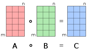
In mathematics, the Hadamard product is a binary operation that takes in two matrices of the same dimensions and returns a matrix of the multiplied corresponding elements. This operation can be thought as a "naive matrix multiplication" and is different from the matrix product. It is attributed to, and named after, either French mathematician Jacques Hadamard or German mathematician Issai Schur.

In mathematics, the Khatri–Rao product or block Kronecker product of two partitioned matrices $and is defined as$

This page is based on this Wikipedia article
Text is available under the CC BY-SA 4.0 license; additional terms may apply.
Images, videos and audio are available under their respective licenses.

[1] B. Berggren, "Pytagoreiska trianglar" (in Swedish), Elementa: Tidskrift för elementär matematik, fysik och kemi 17 (1934), 129–139. See page 6 for the rooted tree.

[2] Barning, F. J. M. (1963), "Over pythagorese en bijna-pythagorese driehoeken en een generatieproces met behulp van unimodulaire matrices" (in Dutch), Math. Centrum Amsterdam Afd. Zuivere Wisk. ZW-011: 37, https://ir.cwi.nl/pub/7151

[3] A. Hall, "Genealogy of Pythagorean Triads", The Mathematical Gazette , volume 54, number 390, December, 1970, pages 377–9.

[4] Kanga, A. R., "The family tree of Pythagorean triples," Bulletin of the Institute of Mathematics and its Applications 26, January/February 1990, 15–17.

[5] Firstov, V. E. (2008). "A Special Matrix Transformation Semigroup of Primitive Pairs and the Genealogy of Pythagorean Triples". Mat. Zametki. 84 (2): 281–299. doi: 10.4213/mzm4074 .

[Price-6] 1 2 Price, H. Lee (2008). "The Pythagorean Tree: A New Species". arXiv: 0809.4324 [math.HO].

[7] Mitchell, Douglas W., "Feedback on 92.60", Mathematical Gazette 93, July 2009, 358–9.

[8] Saunders, Robert A.; Randall, Trevor (July 1994), "The family tree of the Pythagorean triplets revisited", Mathematical Gazette, 78: 190–193, doi:10.2307/3618576, JSTOR 3618576, S2CID 125749577 .

[9] Mitchell, Douglas W., "An alternative characterisation of all primitive Pythagorean triples", Mathematical Gazette 85, July 2001, 273–275.

[1]

[2]

[3]

[4]

[5]

[6]

[7]

[8]

[9]