For matrix multiplication, the number of columns in the first matrix must be equal to the number of rows in the second matrix. The result matrix has the number of rows of the first and the number of columns of the second matrix.
In mathematics, particularly in linear algebra, matrix multiplication is a binary operation that produces a matrix from two matrices. For matrix multiplication, the number of columns in the first matrix must be equal to the number of rows in the second matrix. The resulting matrix, known as the matrix product, has the number of rows of the first and the number of columns of the second matrix. The product of matrices A and B is denoted as AB.[1]
This article will use the following notational conventions: matrices are represented by capital letters in bold, e.g. A; vectors in lowercase bold, e.g. a; and entries of vectors and matrices are italic (they are numbers from a field), e.g. A and a. Index notation is often the clearest way to express definitions, and is used as standard in the literature. The entry in row i, column j of matrix A is indicated by (A)ij, Aij or aij. In contrast, a single subscript, e.g. A1, A2, is used to select a matrix (not a matrix entry) from a collection of matrices.
Definitions
Matrix times matrix
If A is an m × n matrix and B is an n × p matrix,
the matrix productC = AB (denoted without multiplication signs or dots) is defined to be the m × p matrix[5][6][7][8]
such that
for i = 1, ..., m and j = 1, ..., p.
That is, the entry of the product is obtained by multiplying term-by-term the entries of the ith row of A and the jth column of B, and summing these n products. In other words, is the dot product of the ith row of A and the jth column of B.
Therefore, AB can also be written as
Thus the product AB is defined if and only if the number of columns in A equals the number of rows in B,[1] in this case n.
In most scenarios, the entries are numbers, but they may be any kind of mathematical objects for which an addition and a multiplication are defined, that are associative, and such that the addition is commutative, and the multiplication is distributive with respect to the addition. In particular, the entries may be matrices themselves (see block matrix).
Matrix times vector
A vector of length can be viewed as a column vector, corresponding to an matrix whose entries are given by If is an matrix, the matrix-times-vector product denoted by is then the vector that, viewed as a column vector, is equal to the matrix In index notation, this amounts to:
One way of looking at this is that the changes from "plain" vector to column vector and back are assumed and left implicit.
Vector times matrix
Similarly, a vector of length can be viewed as a row vector, corresponding to a matrix. To make it clear that a row vector is meant, it is customary in this context to represent it as the transpose of a column vector; thus, one will see notations such as The identity holds. In index notation, if is an matrix, amounts to:
Vector times vector
The dot product of two vectors and of equal length is equal to the single entry of the matrix resulting from multiplying these vectors as a row and a column vector, thus: (or which results in the same matrix).
Illustration
The figure to the right illustrates diagrammatically the product of two matrices A and B, showing how each intersection in the product matrix corresponds to a row of A and a column of B.
The values at the intersections, marked with circles in figure to the right, are:
Fundamental applications
Historically, matrix multiplication has been introduced for facilitating and clarifying computations in linear algebra. This strong relationship between matrix multiplication and linear algebra remains fundamental in all mathematics, as well as in physics, chemistry, engineering and computer science.
Linear maps
If a vector space has a finite basis, its vectors are each uniquely represented by a finite sequence of scalars, called a coordinate vector, whose elements are the coordinates of the vector on the basis. These coordinate vectors form another vector space, which is isomorphic to the original vector space. A coordinate vector is commonly organized as a column matrix (also called a column vector), which is a matrix with only one column. So, a column vector represents both a coordinate vector, and a vector of the original vector space.
A linear mapA from a vector space of dimension n into a vector space of dimension m maps a column vector
onto the column vector
The linear map A is thus defined by the matrix
and maps the column vector to the matrix product
If B is another linear map from the preceding vector space of dimension m, into a vector space of dimension p, it is represented by a matrix A straightforward computation shows that the matrix of the composite map is the matrix product The general formula ) that defines the function composition is instanced here as a specific case of associativity of matrix product (see §Associativity below):
where the source point and its image are written as column vectors.
The composition of the rotation by and that by then corresponds to the matrix product
where appropriate trigonometric identities are employed for the second equality. That is, the composition corresponds to the rotation by angle , as expected.
Resource allocation in economics
The computation of the bottom left entry of corresponds to the consideration of all paths (highlighted) from basic commodity to final product in the production flow graph.
provide the amount of basic commodities needed for a given amount of intermediate goods, and the amount of intermediate goods needed for a given amount of final products, respectively. For example, to produce one unit of intermediate good , one unit of basic commodity , two units of , no units of , and one unit of are needed, corresponding to the first column of .
Using matrix multiplication, compute
this matrix directly provides the amounts of basic commodities needed for given amounts of final goods. For example, the bottom left entry of is computed as , reflecting that units of are needed to produce one unit of . Indeed, one unit is needed for , one for each of two , and for each of the four units that go into the unit, see picture.
In order to produce e.g. 100 units of the final product , 80 units of , and 60 units of , the necessary amounts of basic goods can be computed as
that is, units of , units of , units of , units of are needed. Similarly, the product matrix can be used to compute the needed amounts of basic goods for other final-good amount data.[9]
where denotes the conjugate transpose of (conjugate of the transpose, or equivalently transpose of the conjugate).
General properties
Matrix multiplication shares some properties with usual multiplication. However, matrix multiplication is not defined if the number of columns of the first factor differs from the number of rows of the second factor, and it is non-commutative,[10] even when the product remains defined after changing the order of the factors.[11][12]
Non-commutativity
An operation is commutative if, given two elements A and B such that the product is defined, then is also defined, and
If A and B are matrices of respective sizes and , then is defined if , and is defined if . Therefore, if one of the products is defined, the other one need not be defined. If , the two products are defined, but have different sizes; thus they cannot be equal. Only if , that is, if A and B are square matrices of the same size, are both products defined and of the same size. Even in this case, one has in general
For example
but
This example may be expanded for showing that, if A is a matrix with entries in a fieldF, then for every matrix B with entries in F, if and only if where , and I is the identity matrix. If, instead of a field, the entries are supposed to belong to a ring, then one must add the condition that c belongs to the center of the ring.
One special case where commutativity does occur is when D and E are two (square) diagonal matrices (of the same size); then DE = ED.[10] Again, if the matrices are over a general ring rather than a field, the corresponding entries in each must also commute with each other for this to hold.
Distributivity
The matrix product is distributive with respect to matrix addition. That is, if A, B, C, D are matrices of respective sizes m × n, n × p, n × p, and p × q, one has (left distributivity)
This results from the distributivity for coefficients by
Product with a scalar
If A is a matrix and c a scalar, then the matrices and are obtained by left or right multiplying all entries of A by c. If the scalars have the commutative property, then
If the product is defined (that is, the number of columns of A equals the number of rows of B), then
and
If the scalars have the commutative property, then all four matrices are equal. More generally, all four are equal if c belongs to the center of a ring containing the entries of the matrices, because in this case, cX = Xc for all matrices X.
These properties result from the bilinearity of the product of scalars:
Transpose
If the scalars have the commutative property, the transpose of a product of matrices is the product, in the reverse order, of the transposes of the factors. That is
where T denotes the transpose, that is the interchange of rows and columns.
This identity does not hold for noncommutative entries, since the order between the entries of A and B is reversed, when one expands the definition of the matrix product.
This results from applying to the definition of matrix product the fact that the conjugate of a sum is the sum of the conjugates of the summands and the conjugate of a product is the product of the conjugates of the factors.
Transposition acts on the indices of the entries, while conjugation acts independently on the entries themselves. It results that, if A and B have complex entries, one has
where † denotes the conjugate transpose (conjugate of the transpose, or equivalently transpose of the conjugate).
Associativity
Given three matrices A, B and C, the products (AB)C and A(BC) are defined if and only if the number of columns of A equals the number of rows of B, and the number of columns of B equals the number of rows of C (in particular, if one of the products is defined, then the other is also defined). In this case, one has the associative property
As for any associative operation, this allows omitting parentheses, and writing the above products as
This extends naturally to the product of any number of matrices provided that the dimensions match. That is, if A1, A2, ..., An are matrices such that the number of columns of Ai equals the number of rows of Ai + 1 for i = 1, ..., n – 1, then the product
These properties may be proved by straightforward but complicated summation manipulations. This result also follows from the fact that matrices represent linear maps. Therefore, the associative property of matrices is simply a specific case of the associative property of function composition.
Computational complexity depends on parenthezation
Although the result of a sequence of matrix products does not depend on the order of operation (provided that the order of the matrices is not changed), the computational complexity may depend dramatically on this order.
For example, if A, B and C are matrices of respective sizes 10×30, 30×5, 5×60, computing (AB)C needs 10×30×5 + 10×5×60 = 4,500 multiplications, while computing A(BC) needs 30×5×60 + 10×30×60 = 27,000 multiplications.
Algorithms have been designed for choosing the best order of products, see Matrix chain multiplication. When the number n of matrices increases, it has been shown that the choice of the best order has a complexity of
Similarity transformations map product to products, that is
In fact, one has
Square matrices
Let us denote the set of n×nsquare matrices with entries in a ringR, which, in practice, is often a field.
In , the product is defined for every pair of matrices. This makes a ring, which has the identity matrixI as identity element (the matrix whose diagonal entries are equal to 1 and all other entries are 0). This ring is also an associative R-algebra.
If n > 1, many matrices do not have a multiplicative inverse. For example, a matrix such that all entries of a row (or a column) are 0 does not have an inverse. If it exists, the inverse of a matrix A is denoted A−1, and, thus verifies
A product of matrices is invertible if and only if each factor is invertible. In this case, one has
When R is commutative, and, in particular, when it is a field, the determinant of a product is the product of the determinants. As determinants are scalars, and scalars commute, one has thus
The other matrix invariants do not behave as well with products. Nevertheless, if R is commutative, AB and BA have the same trace, the same characteristic polynomial, and the same eigenvalues with the same multiplicities. However, the eigenvectors are generally different if AB ≠ BA.
Powers of a matrix
One may raise a square matrix to any nonnegative integer power multiplying it by itself repeatedly in the same way as for ordinary numbers. That is,
Computing the kth power of a matrix needs k – 1 times the time of a single matrix multiplication, if it is done with the trivial algorithm (repeated multiplication). As this may be very time consuming, one generally prefers using exponentiation by squaring, which requires less than 2 log2k matrix multiplications, and is therefore much more efficient.
An easy case for exponentiation is that of a diagonal matrix. Since the product of diagonal matrices amounts to simply multiplying corresponding diagonal elements together, the kth power of a diagonal matrix is obtained by raising the entries to the power k:
Abstract algebra
The definition of matrix product requires that the entries belong to a semiring, and does not require multiplication of elements of the semiring to be commutative. In many applications, the matrix elements belong to a field, although the tropical semiring is also a common choice for graph shortest path problems.[13] Even in the case of matrices over fields, the product is not commutative in general, although it is associative and is distributive over matrix addition. The identity matrices (which are the square matrices whose entries are zero outside of the main diagonal and 1 on the main diagonal) are identity elements of the matrix product. It follows that the n × n matrices over a ring form a ring, which is noncommutative except if n = 1 and the ground ring is commutative.
A square matrix may have a multiplicative inverse, called an inverse matrix. In the common case where the entries belong to a commutative ringR, a matrix has an inverse if and only if its determinant has a multiplicative inverse in R. The determinant of a product of square matrices is the product of the determinants of the factors. The n × n matrices that have an inverse form a group under matrix multiplication, the subgroups of which are called matrix groups. Many classical groups (including all finite groups) are isomorphic to matrix groups; this is the starting point of the theory of group representations.
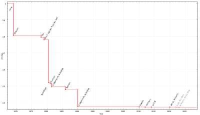
Improvement of estimates of exponent ω over time for the computational complexity of matrix multiplication
The matrix multiplication algorithm that results from the definition requires, in the worst case, multiplications and additions of scalars to compute the product of two square n×n matrices. Its computational complexity is therefore , in a model of computation for which the scalar operations take constant time.
Rather surprisingly, this complexity is not optimal, as shown in 1969 by Volker Strassen, who provided an algorithm, now called Strassen's algorithm, with a complexity of [14] Strassen's algorithm can be parallelized to further improve the performance.[15]As of January2024[update], the best peer-reviewed matrix multiplication algorithm is by Virginia Vassilevska Williams, Yinzhan Xu, Zixuan Xu, and Renfei Zhou and has complexity O(n2.371552).[16][17] It is not known whether matrix multiplication can be performed in n2 + o(1) time.[18] This would be optimal, since one must read the elements of a matrix in order to multiply it with another matrix.
Since matrix multiplication forms the basis for many algorithms, and many operations on matrices even have the same complexity as matrix multiplication (up to a multiplicative constant), the computational complexity of matrix multiplication appears throughout numerical linear algebra and theoretical computer science.
↑ Adams, R. A. (1995). Calculus, A Complete Course (3rded.). Addison Wesley. p.627. ISBN0-201-82823-5.
↑ Horn, Johnson (2013). Matrix Analysis (2nded.). Cambridge University Press. p.6. ISBN978-0-521-54823-6.
↑ Peter Stingl (1996). Mathematik für Fachhochschulen – Technik und Informatik (in German) (5thed.). Munich: Carl Hanser Verlag. ISBN3-446-18668-9. Here: Exm.5.4.10, p.205-206
↑ Vassilevska Williams, Virginia; Xu, Yinzhan; Xu, Zixuan; Zhou, Renfei. New Bounds for Matrix Multiplication: from Alpha to Omega. Proceedings of the 2024 Annual ACM-SIAM Symposium on Discrete Algorithms (SODA). pp.3792–3835. arXiv:2307.07970. doi:10.1137/1.9781611977912.134.
↑ that is, in time n2+f(n), for some function f with f(n)→0 as n→∞
Related Research Articles
In mathematics, the determinant is a scalar value that is a certain function of the entries of a square matrix. The determinant of a matrix A is commonly denoted det(A), det A, or |A|. Its value characterizes some properties of the matrix and the linear map represented, on a given basis, by the matrix. In particular, the determinant is nonzero if and only if the matrix is invertible and the corresponding linear map is an isomorphism. The determinant of a product of matrices is the product of their determinants.
In mathematics, and more specifically in linear algebra, a linear map is a mapping between two vector spaces that preserves the operations of vector addition and scalar multiplication. The same names and the same definition are also used for the more general case of modules over a ring; see Module homomorphism.
In mathematical physics and mathematics, the Pauli matrices are a set of three 2 × 2 complex matrices that are Hermitian, involutory and unitary. Usually indicated by the Greek letter sigma, they are occasionally denoted by tau when used in connection with isospin symmetries.
In linear algebra, the outer product of two coordinate vectors is the matrix whose entries are all products of an element in the first vector with an element in the second vector. If the two coordinate vectors have dimensions n and m, then their outer product is an n × m matrix. More generally, given two tensors, their outer product is a tensor. The outer product of tensors is also referred to as their tensor product, and can be used to define the tensor algebra.
In linear algebra, an orthogonal matrix, or orthonormal matrix, is a real square matrix whose columns and rows are orthonormal vectors.
In linear algebra, the Cayley–Hamilton theorem states that every square matrix over a commutative ring satisfies its own characteristic equation.
In mechanics and geometry, the 3D rotation group, often denoted SO(3), is the group of all rotations about the origin of three-dimensional Euclidean space under the operation of composition.
Unit quaternions, known as versors, provide a convenient mathematical notation for representing spatial orientations and rotations of elements in three dimensional space. Specifically, they encode information about an axis-angle rotation about an arbitrary axis. Rotation and orientation quaternions have applications in computer graphics, computer vision, robotics, navigation, molecular dynamics, flight dynamics, orbital mechanics of satellites, and crystallographic texture analysis.
In linear algebra, an n-by-n square matrix A is called invertible if there exists an n-by-n square matrix B such that
In mathematics, the conjugate transpose, also known as the Hermitian transpose, of an complex matrix is an matrix obtained by transposing and applying complex conjugation to each entry. There are several notations, such as or , , or .
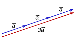
In mathematics, scalar multiplication is one of the basic operations defining a vector space in linear algebra. In common geometrical contexts, scalar multiplication of a real Euclidean vector by a positive real number multiplies the magnitude of the vector without changing its direction. Scalar multiplication is the multiplication of a vector by a scalar, and is to be distinguished from inner product of two vectors.
In linear algebra, a QR decomposition, also known as a QR factorization or QU factorization, is a decomposition of a matrix A into a product A = QR of an orthonormal matrix Q and an upper triangular matrix R. QR decomposition is often used to solve the linear least squares (LLS) problem and is the basis for a particular eigenvalue algorithm, the QR algorithm.
In mathematics, a block matrix or a partitioned matrix is a matrix that is interpreted as having been broken into sections called blocks or submatrices.
In numerical linear algebra, a Givens rotation is a rotation in the plane spanned by two coordinates axes. Givens rotations are named after Wallace Givens, who introduced them to numerical analysts in the 1950s while he was working at Argonne National Laboratory.
In linear algebra, linear transformations can be represented by matrices. If is a linear transformation mapping to and is a column vector with entries, then
In mathematics, the Kronecker product, sometimes denoted by ⊗, is an operation on two matrices of arbitrary size resulting in a block matrix. It is a specialization of the tensor product from vectors to matrices and gives the matrix of the tensor product linear map with respect to a standard choice of basis. The Kronecker product is to be distinguished from the usual matrix multiplication, which is an entirely different operation. The Kronecker product is also sometimes called matrix direct product.
In linear algebra, a rotation matrix is a transformation matrix that is used to perform a rotation in Euclidean space. For example, using the convention below, the matrix
In linear algebra, a circulant matrix is a square matrix in which all rows are composed of the same elements and each row is rotated one element to the right relative to the preceding row. It is a particular kind of Toeplitz matrix.
In mathematics, the Smith normal form is a normal form that can be defined for any matrix with entries in a principal ideal domain (PID). The Smith normal form of a matrix is diagonal, and can be obtained from the original matrix by multiplying on the left and right by invertible square matrices. In particular, the integers are a PID, so one can always calculate the Smith normal form of an integer matrix. The Smith normal form is very useful for working with finitely generated modules over a PID, and in particular for deducing the structure of a quotient of a free module. It is named after the Irish mathematician Henry John Stephen Smith.
In mathematics, specifically multilinear algebra, a dyadic or dyadic tensor is a second order tensor, written in a notation that fits in with vector algebra.
Henry Cohn, Robert Kleinberg, Balázs Szegedy, and Chris Umans. Group-theoretic Algorithms for Matrix Multiplication. arXiv:math.GR/0511460. Proceedings of the 46th Annual Symposium on Foundations of Computer Science, 23–25 October 2005, Pittsburgh, PA, IEEE Computer Society, pp.379–388.
Henry Cohn, Chris Umans. A Group-theoretic Approach to Fast Matrix Multiplication. arXiv:math.GR/0307321. Proceedings of the 44th Annual IEEE Symposium on Foundations of Computer Science, 11–14 October 2003, Cambridge, MA, IEEE Computer Society, pp.438–449.
Ran Raz. On the complexity of matrix product. In Proceedings of the thirty-fourth annual ACM symposium on Theory of computing. ACM Press, 2002. doi:10.1145/509907.509932.
Robinson, Sara, Toward an Optimal Algorithm for Matrix Multiplication, SIAM News 38(9), November 2005. PDF
Strassen, Volker, Gaussian Elimination is not Optimal, Numer. Math. 13, p.354–356, 1969.
This page is based on this Wikipedia article Text is available under the CC BY-SA 4.0 license; additional terms may apply. Images, videos and audio are available under their respective licenses.