
In physics and engineering, fluid dynamics is a subdiscipline of fluid mechanics that describes the flow of fluids—liquids and gases. It has several subdisciplines, including aerodynamics and hydrodynamics. Fluid dynamics has a wide range of applications, including calculating forces and moments on aircraft, determining the mass flow rate of petroleum through pipelines, predicting weather patterns, understanding nebulae in interstellar space and modelling fission weapon detonation.

In fluid dynamics, laminar flow is characterized by fluid particles following smooth paths in layers, with each layer moving smoothly past the adjacent layers with little or no mixing. At low velocities, the fluid tends to flow without lateral mixing, and adjacent layers slide past one another like playing cards. There are no cross-currents perpendicular to the direction of flow, nor eddies or swirls of fluids. In laminar flow, the motion of the particles of the fluid is very orderly with particles close to a solid surface moving in straight lines parallel to that surface. Laminar flow is a flow regime characterized by high momentum diffusion and low momentum convection.
In fluid dynamics, turbulence or turbulent flow is fluid motion characterized by chaotic changes in pressure and flow velocity. It is in contrast to a laminar flow, which occurs when a fluid flows in parallel layers, with no disruption between those layers.

In fluid dynamics, a vortex is a region in a fluid in which the flow revolves around an axis line, which may be straight or curved. Vortices form in stirred fluids, and may be observed in smoke rings, whirlpools in the wake of a boat, and the winds surrounding a tropical cyclone, tornado or dust devil.
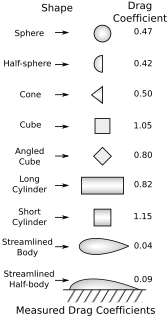
In fluid dynamics, the drag coefficient is a dimensionless quantity that is used to quantify the drag or resistance of an object in a fluid environment, such as air or water. It is used in the drag equation in which a lower drag coefficient indicates the object will have less aerodynamic or hydrodynamic drag. The drag coefficient is always associated with a particular surface area.

In physics and fluid mechanics, a boundary layer is the layer of fluid in the immediate vicinity of a bounding surface where the effects of viscosity are significant. The liquid or gas in the boundary layer tends to cling to the surface.

An airfoil or aerofoil is the cross-sectional shape of an object whose motion through a gas is capable of generating significant lift, such as a wing, a sail, or the blades of propeller, rotor, or turbine.

Parasitic drag is drag that acts on an object when the object is moving through a fluid. In the case of aerodynamic drag, the fluid is the atmosphere. Parasitic drag is a combination of form drag and skin friction drag. Parasitic drag does not result from the generation of lift on the object, and hence it is considered parasitic.
Boundary layer control refers to methods of controlling the behaviour of fluid flow boundary layers.

In fluid dynamics, an eddy is the swirling of a fluid and the reverse current created when the fluid is in a turbulent flow regime. The moving fluid creates a space devoid of downstream-flowing fluid on the downstream side of the object. Fluid behind the obstacle flows into the void creating a swirl of fluid on each edge of the obstacle, followed by a short reverse flow of fluid behind the obstacle flowing upstream, toward the back of the obstacle. This phenomenon is naturally observed behind large emergent rocks in swift-flowing rivers.

Whenever there is relative movement between a fluid and a solid surface, whether externally round a body, or internally in an enclosed passage, a boundary layer exists with viscous forces present in the layer of fluid close to the surface. Boundary layers can be either laminar or turbulent. A reasonable assessment of whether the boundary layer will be laminar or turbulent can be made by calculating the Reynolds number of the local flow conditions.
This page describes some of the parameters used to characterize the thickness and shape of boundary layers formed by fluid flowing along a solid surface. The defining characteristic of boundary layer flow is that at the solid walls, the fluid's velocity is reduced to zero. The boundary layer refers to the thin transition layer between the wall and the bulk fluid flow. The boundary layer concept was originally developed by Ludwig Prandtl and is broadly classified into two types, bounded and unbounded. Each of the main types has a laminar, transitional, and turbulent sub-type. The two types of boundary layers use similar methods to describe the thickness and shape of the transition region with a couple of exceptions detailed in the Unbounded Boundary Layer Section. The characterizations detailed below consider steady flow but is easily extended to unsteady flow.
In fluid dynamics, flow can be decomposed into primary plus secondary flow, a relatively weaker flow pattern superimposed on the stronger primary flow pattern. The primary flow is often chosen to be an exact solution to simplified or approximated governing equations, such as potential flow around a wing or geostrophic current or wind on the rotating Earth. In that case, the secondary flow usefully spotlights the effects of complicated real-world terms neglected in those approximated equations. For instance, the consequences of viscosity are spotlighted by secondary flow in the viscous boundary layer, resolving the tea leaf paradox. As another example, if the primary flow is taken to be a balanced flow approximation with net force equated to zero, then the secondary circulation helps spotlight acceleration due to the mild imbalance of forces. A smallness assumption about secondary flow also facilitates linearization.
In fluid dynamics, a Tollmien–Schlichting wave is a streamwise unstable wave which arises in a bounded shear flow. It is one of the more common methods by which a laminar bounded shear flow transitions to turbulence. The waves are initiated when some disturbance interacts with leading edge roughness in a process known as receptivity. These waves are slowly amplified as they move downstream until they may eventually grow large enough that nonlinearities take over and the flow transitions to turbulence.

The Reynolds number helps predict flow patterns in different fluid flow situations. At low Reynolds numbers, flows tend to be dominated by laminar (sheet-like) flow, while at high Reynolds numbers flows tend to be turbulent. The turbulence results from differences in the fluid's speed and direction, which may sometimes intersect or even move counter to the overall direction of the flow. These eddy currents begin to churn the flow, using up energy in the process, which for liquids increases the chances of cavitation. Reynolds numbers are an important dimensionless quantity in fluid mechanics.
In engineering, physics and chemistry, the study of transport phenomena concerns the exchange of mass, energy, charge, momentum and angular momentum between observed and studied systems. While it draws from fields as diverse as continuum mechanics and thermodynamics, it places a heavy emphasis on the commonalities between the topics covered. Mass, momentum, and heat transport all share a very similar mathematical framework, and the parallels between them are exploited in the study of transport phenomena to draw deep mathematical connections that often provide very useful tools in the analysis of one field that are directly derived from the others.

Almost every computational fluid dynamics problem is defined under the limits of initial and boundary conditions. When constructing a staggered grid, it is common to implement boundary conditions by adding an extra node across the physical boundary. The nodes just outside the inlet of the system are used to assign the inlet conditions and the physical boundaries can coincide with the scalar control volume boundaries. This makes it possible to introduce the boundary conditions and achieve discrete equations for nodes near the boundaries with small modifications.
K-epsilon (k-ε) turbulence model is the most common model used in Computational Fluid Dynamics (CFD) to simulate mean flow characteristics for turbulent flow conditions. It is a two equation model that gives a general description of turbulence by means of two transport equations (PDEs). The original impetus for the K-epsilon model was to improve the mixing-length model, as well as to find an alternative to algebraically prescribing turbulent length scales in moderate to high complexity flows.
In fluid dynamics, the entrance length is the distance a flow travels after entering a pipe before the flow becomes fully developed. Entrance length refers to the length of the entry region, the area following the pipe entrance where effects originating from the interior wall of the pipe propagate into the flow as an expanding boundary layer. When the boundary layer expands to fill the entire pipe, the developing flow becomes a fully developed flow, where flow characteristics no longer change with increased distance along the pipe. Many different entrance lengths exist to describe a variety of flow conditions. Hydrodynamic entrance length describes the formation of a velocity profile caused by viscous forces propagating from the pipe wall. Thermal entrance length describes the formation of a temperature profile. Awareness of entrance length may be necessary for the effective placement of instrumentation, such as fluid flow meters.
Skin friction drag is a component of parasitic drag, which is resistant force exerted on an object moving in a fluid. Skin friction drag is caused by the viscosity of fluids and is developed from laminar drag to turbulent drag as a fluid moves on the surface of an object. Skin friction drag is generally expressed in terms of the Reynolds number, which is the ratio between inertial force and viscous force.

