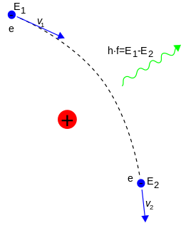
Bremsstrahlung, from bremsen "to brake" and Strahlung "radiation"; i.e., "braking radiation" or "deceleration radiation", is electromagnetic radiation produced by the deceleration of a charged particle when deflected by another charged particle, typically an electron by an atomic nucleus. The moving particle loses kinetic energy, which is converted into radiation, thus satisfying the law of conservation of energy. The term is also used to refer to the process of producing the radiation. Bremsstrahlung has a continuous spectrum, which becomes more intense and whose peak intensity shifts toward higher frequencies as the change of the energy of the decelerated particles increases.
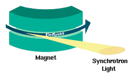
Synchrotron radiation is the electromagnetic radiation emitted when charged particles are accelerated radially, i.e., when they are subject to an acceleration perpendicular to their velocity. It is produced, for example, in synchrotrons using bending magnets, undulators and/or wigglers. If the particle is non-relativistic, then the emission is called cyclotron emission. If, on the other hand, the particles are relativistic, sometimes referred to as ultrarelativistic, the emission is called synchrotron emission. Synchrotron radiation may be achieved artificially in synchrotrons or storage rings, or naturally by fast electrons moving through magnetic fields. The radiation produced in this way has a characteristic polarization and the frequencies generated can range over the entire electromagnetic spectrum which is also called continuum radiation.
Linear elasticity is a mathematical model of how solid objects deform and become internally stressed due to prescribed loading conditions. It is a simplification of the more general nonlinear theory of elasticity and a branch of continuum mechanics.

In physics, the Rabi cycle is the cyclic behaviour of a two-level quantum system in the presence of an oscillatory driving field. A great variety of physical processes belonging to the areas of quantum computing, condensed matter, atomic and molecular physics, and nuclear and particle physics can be conveniently studied in terms of two-level quantum mechanical systems, and exhibit Rabi flopping when coupled to an oscillatory driving field. The effect is important in quantum optics, magnetic resonance and quantum computing, and is named after Isidor Isaac Rabi.
In physics, a wave vector is a vector which helps describe a wave. Like any vector, it has a magnitude and direction, both of which are important: Its magnitude is either the wavenumber or angular wavenumber of the wave, and its direction is ordinarily the direction of wave propagation.
In mathematics, the Hamilton–Jacobi equation (HJE) is a necessary condition describing extremal geometry in generalizations of problems from the calculus of variations, and is a special case of the Hamilton–Jacobi–Bellman equation. It is named for William Rowan Hamilton and Carl Gustav Jacob Jacobi.
The rigid rotor is a mechanical model of rotating systems. An arbitrary rigid rotor is a 3-dimensional rigid object, such as a top. To orient such an object in space requires three angles, known as Euler angles. A special rigid rotor is the linear rotor requiring only two angles to describe, for example of a diatomic molecule. More general molecules are 3-dimensional, such as water, ammonia, or methane.
In fluid dynamics, Couette flow is the flow of a viscous fluid in the space between two surfaces, one of which is moving tangentially relative to the other. The configuration often takes the form of two parallel plates or the gap between two concentric cylinders. The flow is driven by virtue of viscous drag force acting on the fluid, but may additionally be motivated by an applied pressure gradient in the flow direction. The Couette configuration models certain practical problems, like flow in lightly loaded journal bearings, and is often employed in viscometry and to demonstrate approximations of reversibility. This type of flow is named in honor of Maurice Couette, a Professor of Physics at the French University of Angers in the late 19th century.
In physics, spherically symmetric spacetimes are commonly used to obtain analytic and numerical solutions to Einstein's field equations in the presence of radially-moving dust, compressible and incompressible fluids or baryons (hydrogen). Because spherically symmetric spacetimes are by definition irrotational, they are not realistic models of black holes in nature; however, the sphere symmetry allows a metric of a considerably simpler form than that of a rotating spacetime, making sphere-symmetric problems much easier to solve. Such models are not entirely inappropriate: they often have a Penrose diagram similar to a rotating spacetime, and so typically have qualitative features that carry on to rotating spacetimes. One such application is the study of mass inflation due to counter-moving streams of infalling matter in the interior of a black hole.
The electromagnetic wave equation is a second-order partial differential equation that describes the propagation of electromagnetic waves through a medium or in a vacuum. It is a three-dimensional form of the wave equation. The homogeneous form of the equation, written in terms of either the electric field E or the magnetic field B, takes the form:

A theoretical motivation for general relativity, including the motivation for the geodesic equation and the Einstein field equation, can be obtained from special relativity by examining the dynamics of particles in circular orbits about the earth. A key advantage in examining circular orbits is that it is possible to know the solution of the Einstein Field Equation a priori. This provides a means to inform and verify the formalism.
A pendulum is a body suspended from a fixed support so that it swings freely back and forth under the influence of gravity. When a pendulum is displaced sideways from its resting, equilibrium position, it is subject to a restoring force due to gravity that will accelerate it back toward the equilibrium position. When released, the restoring force acting on the pendulum's mass causes it to oscillate about the equilibrium position, swinging back and forth. The mathematics of pendulums are in general quite complicated. Simplifying assumptions can be made, which in the case of a simple pendulum allow the equations of motion to be solved analytically for small-angle oscillations.
The history of Lorentz transformations comprises the development of linear transformations forming the Lorentz group or Poincaré group preserving the Lorentz interval and the Minkowski inner product .
Resonance fluorescence is the process in which a two-level atom system interacts with the quantum electromagnetic field if the field is driven at a frequency near to the natural frequency of the atom.
In physics, Berry connection and Berry curvature are related concepts which can be viewed, respectively, as a local gauge potential and gauge field associated with the Berry phase or geometric phase. These concepts were introduced by Michael Berry in a paper published in 1984 emphasizing how geometric phases provide a powerful unifying concept in several branches of classical and quantum physics.
In a paramagnetic material, the magnetization of the material is (approximately) directly proportional to an applied magnetic field. However, if the material is heated, this proportionality is reduced: for a fixed value of the field, the magnetization is (approximately) inversely proportional to temperature. This fact is encapsulated by Curie's law, after Pierre Curie:
Multipole radiation is a theoretical framework for the description of electromagnetic or gravitational radiation from time-dependent distributions of distant sources. These tools are applied to physical phenomena which occur at a variety of length scales - from gravitational waves due to galaxy collisions to gamma radiation resulting from nuclear decay. Multipole radiation is analyzed using similar multipole expansion techniques that describe fields from static sources, however there are important differences in the details of the analysis because multipole radiation fields behave quite differently from static fields. This article is primarily concerned with electromagnetic multipole radiation, although the treatment of gravitational waves is similar.

In statistics, the variance function is a smooth function which depicts the variance of a random quantity as a function of its mean. The variance function plays a large role in many settings of statistical modelling. It is a main ingredient in the generalized linear model framework and a tool used in non-parametric regression, semiparametric regression and functional data analysis. In parametric modeling, variance functions take on a parametric form and explicitly describe the relationship between the variance and the mean of a random quantity. In a non-parametric setting, the variance function is assumed to be a smooth function.
In fluid dynamics, Landau–Squire jet or Submerged Landau jet describes a round submerged jet issued from a point source into an infinite fluid medium of the same kind. This is an exact solution to the Navier-Stokes equations, which was first discovered by Lev Landau in 1944 and later by Herbert Squire in 1951. The self-similar equation was in fact first derived by N. A. Slezkin in 1934, but never applied to the jet. Following Landau's work, V. I. Yatseyev obtained the general solution of the equation in 1950.
The polar form of the Dirac equation writes each of its four spinor components as the product of a module times a unitary complex phase.


