
In mathematics, convolution is a mathematical operation on two functions that produces a third function that expresses how the shape of one is modified by the other. The term convolution refers to both the result function and to the process of computing it. It is defined as the integral of the product of the two functions after one is reflected about the y-axis and shifted. The choice of which function is reflected and shifted before the integral does not change the integral result. The integral is evaluated for all values of shift, producing the convolution function.
In engineering, a transfer function of a system, sub-system, or component is a mathematical function that theoretically models the system's output for each possible input. They are widely used in electronics and control systems. In some simple cases, this function is a two-dimensional graph of an independent scalar input versus the dependent scalar output, called a transfer curve or characteristic curve. Transfer functions for components are used to design and analyze systems assembled from components, particularly using the block diagram technique, in electronics and control theory.
In signal processing, group delay and phase delay are delay times experienced by a signal's various frequency components when the signal passes through a linear time-invariant system (LTI), such as a microphone, coaxial cable, amplifier, loudspeaker, telecommunications system or ethernet cable. These delays are generally frequency dependent, which means that different frequency components experience different delays. As a result, the signal's waveform experiences distortion as it passes through the system. This distortion can cause problems such as poor fidelity in analog video and analog audio, or a high bit-error rate in a digital bit stream. For a modulation signal, the information carried by the signal is carried exclusively in the wave envelope. Group delay therefore operates only with the frequency components derived from the envelope.

In physics and mathematics, the Fourier transform (FT) is a transform that converts a function into a form that describes the frequencies present in the original function. The output of the transform is a complex-valued function of frequency. The term Fourier transform refers to both this complex-valued function and the mathematical operation. When a distinction needs to be made the Fourier transform is sometimes called the frequency domain representation of the original function. The Fourier transform is analogous to decomposing the sound of a musical chord into terms of the intensity of its constituent pitches.
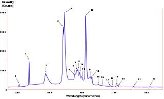
The power spectrum of a time series describes the distribution of power into frequency components composing that signal. According to Fourier analysis, any physical signal can be decomposed into a number of discrete frequencies, or a spectrum of frequencies over a continuous range. The statistical average of a certain signal or sort of signal as analyzed in terms of its frequency content, is called its spectrum.
Analog signal processing is a type of signal processing conducted on continuous analog signals by some analog means. "Analog" indicates something that is mathematically represented as a set of continuous values. This differs from "digital" which uses a series of discrete quantities to represent signal. Analog values are typically represented as a voltage, electric current, or electric charge around components in the electronic devices. An error or noise affecting such physical quantities will result in a corresponding error in the signals represented by such physical quantities.

The short-time Fourier transform (STFT), is a Fourier-related transform used to determine the sinusoidal frequency and phase content of local sections of a signal as it changes over time. In practice, the procedure for computing STFTs is to divide a longer time signal into shorter segments of equal length and then compute the Fourier transform separately on each shorter segment. This reveals the Fourier spectrum on each shorter segment. One then usually plots the changing spectra as a function of time, known as a spectrogram or waterfall plot, such as commonly used in software defined radio (SDR) based spectrum displays. Full bandwidth displays covering the whole range of an SDR commonly use fast Fourier transforms (FFTs) with 2^24 points on desktop computers.
In signal processing, a finite impulse response (FIR) filter is a filter whose impulse response is of finite duration, because it settles to zero in finite time. This is in contrast to infinite impulse response (IIR) filters, which may have internal feedback and may continue to respond indefinitely.
In control theory and signal processing, a linear, time-invariant system is said to be minimum-phase if the system and its inverse are causal and stable.
In control theory, a causal system is a system where the output depends on past and current inputs but not future inputs—i.e., the output depends only on the input for values of .
In mathematics and signal processing, the Hilbert transform is a specific singular integral that takes a function, u(t) of a real variable and produces another function of a real variable H(u)(t). The Hilbert transform is given by the Cauchy principal value of the convolution with the function (see § Definition). The Hilbert transform has a particularly simple representation in the frequency domain: It imparts a phase shift of ±90° (π⁄2 radians) to every frequency component of a function, the sign of the shift depending on the sign of the frequency (see § Relationship with the Fourier transform). The Hilbert transform is important in signal processing, where it is a component of the analytic representation of a real-valued signal u(t). The Hilbert transform was first introduced by David Hilbert in this setting, to solve a special case of the Riemann–Hilbert problem for analytic functions.
In signal processing, linear phase is a property of a filter where the phase response of the filter is a linear function of frequency. The result is that all frequency components of the input signal are shifted in time by the same constant amount, which is referred to as the group delay. Consequently, there is no phase distortion due to the time delay of frequencies relative to one another.

In mathematics, a Dirac comb is a periodic function with the formula

In system analysis, among other fields of study, a linear time-invariant (LTI) system is a system that produces an output signal from any input signal subject to the constraints of linearity and time-invariance; these terms are briefly defined below. These properties apply (exactly or approximately) to many important physical systems, in which case the response y(t) of the system to an arbitrary input x(t) can be found directly using convolution: y(t) = (x ∗ h)(t) where h(t) is called the system's impulse response and ∗ represents convolution (not to be confused with multiplication, as is frequently employed by the symbol in computer languages). What's more, there are systematic methods for solving any such system (determining h(t)), whereas systems not meeting both properties are generally more difficult (or impossible) to solve analytically. A good example of an LTI system is any electrical circuit consisting of resistors, capacitors, inductors and linear amplifiers.
A cyclostationary process is a signal having statistical properties that vary cyclically with time. A cyclostationary process can be viewed as multiple interleaved stationary processes. For example, the maximum daily temperature in New York City can be modeled as a cyclostationary process: the maximum temperature on July 21 is statistically different from the temperature on December 20; however, it is a reasonable approximation that the temperature on December 20 of different years has identical statistics. Thus, we can view the random process composed of daily maximum temperatures as 365 interleaved stationary processes, each of which takes on a new value once per year.
In applied mathematics, the Wiener–Khinchin theorem or Wiener–Khintchine theorem, also known as the Wiener–Khinchin–Einstein theorem or the Khinchin–Kolmogorov theorem, states that the autocorrelation function of a wide-sense-stationary random process has a spectral decomposition given by the power spectrum of that process.
In mathematics, a wavelet series is a representation of a square-integrable function by a certain orthonormal series generated by a wavelet. This article provides a formal, mathematical definition of an orthonormal wavelet and of the integral wavelet transform.
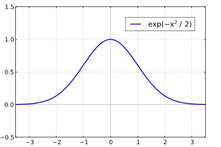
The Gabor transform, named after Dennis Gabor, is a special case of the short-time Fourier transform. It is used to determine the sinusoidal frequency and phase content of local sections of a signal as it changes over time. The function to be transformed is first multiplied by a Gaussian function, which can be regarded as a window function, and the resulting function is then transformed with a Fourier transform to derive the time-frequency analysis. The window function means that the signal near the time being analyzed will have higher weight. The Gabor transform of a signal x(t) is defined by this formula:
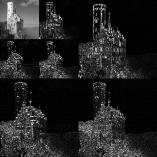
In signal processing, nonlinear multidimensional signal processing (NMSP) covers all signal processing using nonlinear multidimensional signals and systems. Nonlinear multidimensional signal processing is a subset of signal processing (multidimensional signal processing). Nonlinear multi-dimensional systems can be used in a broad range such as imaging, teletraffic, communications, hydrology, geology, and economics. Nonlinear systems cannot be treated as linear systems, using Fourier transformation and wavelet analysis. Nonlinear systems will have chaotic behavior, limit cycle, steady state, bifurcation, multi-stability and so on. Nonlinear systems do not have a canonical representation, like impulse response for linear systems. But there are some efforts to characterize nonlinear systems, such as Volterra and Wiener series using polynomial integrals as the use of those methods naturally extend the signal into multi-dimensions. Another example is the Empirical mode decomposition method using Hilbert transform instead of Fourier Transform for nonlinear multi-dimensional systems. This method is an empirical method and can be directly applied to data sets. Multi-dimensional nonlinear filters (MDNF) are also an important part of NMSP, MDNF are mainly used to filter noise in real data. There are nonlinear-type hybrid filters used in color image processing, nonlinear edge-preserving filters use in magnetic resonance image restoration. Those filters use both temporal and spatial information and combine the maximum likelihood estimate with the spatial smoothing algorithm.
Multidimensional seismic data processing forms a major component of seismic profiling, a technique used in geophysical exploration. The technique itself has various applications, including mapping ocean floors, determining the structure of sediments, mapping subsurface currents and hydrocarbon exploration. Since geophysical data obtained in such techniques is a function of both space and time, multidimensional signal processing techniques may be better suited for processing such data.


