The bilinear transform is used in digital signal processing and discrete-time control theory to transform continuous-time system representations to discrete-time and vice versa.
In mathematics, the Laplace transform, named after its discoverer Pierre-Simon Laplace, is an integral transform that converts a function of a real variable to a function of a complex variable . The transform has many applications in science and engineering, mostly as a tool for solving linear differential equations. In particular, it transforms ordinary differential equations into algebraic equations and convolution into multiplication. For suitable functions f, the Laplace transform is defined by the integral
In engineering, a transfer function of a system, sub-system, or component is a mathematical function that models the system's output for each possible input. It is widely used in electronic engineering tools like circuit simulators and control systems. In simple cases, this function can be represented as a two-dimensional graph of an independent scalar input versus the dependent scalar output. Transfer functions for components are used to design and analyze systems assembled from components, particularly using the block diagram technique, in electronics and control theory.

The uncertainty principle, also known as Heisenberg's indeterminacy principle, is a fundamental concept in quantum mechanics. It states that there is a limit to the precision with which certain pairs of physical properties, such as position and momentum, can be simultaneously known. In other words, the more accurately one property is measured, the less accurately the other property can be known.
In vector calculus, the divergence theorem, also known as Gauss's theorem or Ostrogradsky's theorem, is a theorem which relates the flux of a vector field through a closed surface to the divergence of the field in the volume enclosed.
In mathematics and signal processing, the Z-transform converts a discrete-time signal, which is a sequence of real or complex numbers, into a complex valued frequency-domain representation.

In mathematics, the Weierstrass elliptic functions are elliptic functions that take a particularly simple form. They are named for Karl Weierstrass. This class of functions are also referred to as ℘-functions and they are usually denoted by the symbol ℘, a uniquely fancy script p. They play an important role in the theory of elliptic functions. A ℘-function together with its derivative can be used to parameterize elliptic curves and they generate the field of elliptic functions with respect to a given period lattice.
In control theory and signal processing, a linear, time-invariant system is said to be minimum-phase if the system and its inverse are causal and stable.
In mathematics and signal processing, the Hilbert transform is a specific singular integral that takes a function, u(t) of a real variable and produces another function of a real variable H(u)(t). The Hilbert transform is given by the Cauchy principal value of the convolution with the function (see § Definition). The Hilbert transform has a particularly simple representation in the frequency domain: It imparts a phase shift of ±90° (π/2 radians) to every frequency component of a function, the sign of the shift depending on the sign of the frequency (see § Relationship with the Fourier transform). The Hilbert transform is important in signal processing, where it is a component of the analytic representation of a real-valued signal u(t). The Hilbert transform was first introduced by David Hilbert in this setting, to solve a special case of the Riemann–Hilbert problem for analytic functions.
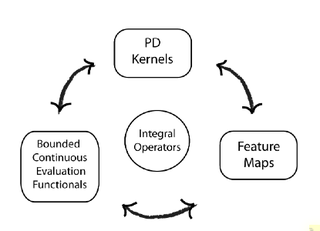
In functional analysis, a reproducing kernel Hilbert space (RKHS) is a Hilbert space of functions in which point evaluation is a continuous linear functional. Roughly speaking, this means that if two functions and in the RKHS are close in norm, i.e., is small, then and are also pointwise close, i.e., is small for all . The converse does not need to be true. Informally, this can be shown by looking at the supremum norm: the sequence of functions converges pointwise, but does not converge uniformly i.e. does not converge with respect to the supremum norm.
In the theory of stochastic processes, the Karhunen–Loève theorem, also known as the Kosambi–Karhunen–Loève theorem states that a stochastic process can be represented as an infinite linear combination of orthogonal functions, analogous to a Fourier series representation of a function on a bounded interval. The transformation is also known as Hotelling transform and eigenvector transform, and is closely related to principal component analysis (PCA) technique widely used in image processing and in data analysis in many fields.

In system analysis, among other fields of study, a linear time-invariant (LTI) system is a system that produces an output signal from any input signal subject to the constraints of linearity and time-invariance; these terms are briefly defined below. These properties apply (exactly or approximately) to many important physical systems, in which case the response y(t) of the system to an arbitrary input x(t) can be found directly using convolution: y(t) = (x ∗ h)(t) where h(t) is called the system's impulse response and ∗ represents convolution (not to be confused with multiplication). What's more, there are systematic methods for solving any such system (determining h(t)), whereas systems not meeting both properties are generally more difficult (or impossible) to solve analytically. A good example of an LTI system is any electrical circuit consisting of resistors, capacitors, inductors and linear amplifiers.
Harmonic balance is a method used to calculate the steady-state response of nonlinear differential equations, and is mostly applied to nonlinear electrical circuits. It is a frequency domain method for calculating the steady state, as opposed to the various time-domain steady-state methods. The name "harmonic balance" is descriptive of the method, which starts with Kirchhoff's Current Law written in the frequency domain and a chosen number of harmonics. A sinusoidal signal applied to a nonlinear component in a system will generate harmonics of the fundamental frequency. Effectively the method assumes a linear combination of sinusoids can represent the solution, then balances current and voltage sinusoids to satisfy Kirchhoff's law. The method is commonly used to simulate circuits which include nonlinear elements, and is most applicable to systems with feedback in which limit cycles occur.
In mathematics, signal processing and control theory, a pole–zero plot is a graphical representation of a rational transfer function in the complex plane which helps to convey certain properties of the system such as:
In mathematics and physics, the Magnus expansion, named after Wilhelm Magnus (1907–1990), provides an exponential representation of the solution of a first-order homogeneous linear differential equation for a linear operator. In particular, it furnishes the fundamental matrix of a system of linear ordinary differential equations of order n with varying coefficients. The exponent is aggregated as an infinite series, whose terms involve multiple integrals and nested commutators.
In mathematical analysis and applications, multidimensional transforms are used to analyze the frequency content of signals in a domain of two or more dimensions.
In signal processing, nonlinear multidimensional signal processing (NMSP) covers all signal processing using nonlinear multidimensional signals and systems. Nonlinear multidimensional signal processing is a subset of signal processing (multidimensional signal processing). Nonlinear multi-dimensional systems can be used in a broad range such as imaging, teletraffic, communications, hydrology, geology, and economics. Nonlinear systems cannot be treated as linear systems, using Fourier transformation and wavelet analysis. Nonlinear systems will have chaotic behavior, limit cycle, steady state, bifurcation, multi-stability and so on. Nonlinear systems do not have a canonical representation, like impulse response for linear systems. But there are some efforts to characterize nonlinear systems, such as Volterra and Wiener series using polynomial integrals as the use of those methods naturally extend the signal into multi-dimensions. Another example is the Empirical mode decomposition method using Hilbert transform instead of Fourier Transform for nonlinear multi-dimensional systems. This method is an empirical method and can be directly applied to data sets. Multi-dimensional nonlinear filters (MDNF) are also an important part of NMSP, MDNF are mainly used to filter noise in real data. There are nonlinear-type hybrid filters used in color image processing, nonlinear edge-preserving filters use in magnetic resonance image restoration. Those filters use both temporal and spatial information and combine the maximum likelihood estimate with the spatial smoothing algorithm.
In mathematics, topological recursion is a recursive definition of invariants of spectral curves. It has applications in enumerative geometry, random matrix theory, mathematical physics, string theory, knot theory.
In functional analysis, every C*-algebra is isomorphic to a subalgebra of the C*-algebra of bounded linear operators on some Hilbert space This article describes the spectral theory of closed normal subalgebras of . A subalgebra of is called normal if it is commutative and closed under the operation: for all , we have and that .
In mathematics, calculus on Euclidean space is a generalization of calculus of functions in one or several variables to calculus of functions on Euclidean space as well as a finite-dimensional real vector space. This calculus is also known as advanced calculus, especially in the United States. It is similar to multivariable calculus but is somewhat more sophisticated in that it uses linear algebra more extensively and covers some concepts from differential geometry such as differential forms and Stokes' formula in terms of differential forms. This extensive use of linear algebra also allows a natural generalization of multivariable calculus to calculus on Banach spaces or topological vector spaces.


