Control theory is a field of control engineering and applied mathematics that deals with the control of dynamical systems in engineered processes and machines. The objective is to develop a model or algorithm governing the application of system inputs to drive the system to a desired state, while minimizing any delay, overshoot, or steady-state error and ensuring a level of control stability; often with the aim to achieve a degree of optimality.
In engineering, a transfer function of a system, sub-system, or component is a mathematical function that models the system's output for each possible input. It is widely used in electronic engineering tools like circuit simulators and control systems. In simple cases, this function can be represented as a two-dimensional graph of an independent scalar input versus the dependent scalar output. Transfer functions for components are used to design and analyze systems assembled from components, particularly using the block diagram technique, in electronics and control theory.
In electronics and control system theory, loop gain is the sum of the gain, expressed as a ratio or in decibels, around a feedback loop. Feedback loops are widely used in electronics in amplifiers and oscillators, and more generally in both electronic and nonelectronic industrial control systems to control industrial plant and equipment. The concept is also used in biology. In a feedback loop, the output of a device, process or plant is sampled and applied to alter the input, to better control the output. The loop gain, along with the related concept of loop phase shift, determines the behavior of the device, and particularly whether the output is stable, or unstable, which can result in oscillation. The importance of loop gain as a parameter for characterizing electronic feedback amplifiers was first recognized by Heinrich Barkhausen in 1921, and was developed further by Hendrik Wade Bode and Harry Nyquist at Bell Labs in the 1930s.
A proportional–integral–derivative controller is a control loop mechanism employing feedback that is widely used in industrial control systems and a variety of other applications requiring continuously modulated control. A PID controller continuously calculates an error value as the difference between a desired setpoint (SP) and a measured process variable (PV) and applies a correction based on proportional, integral, and derivative terms, hence the name.

In electrical engineering and control theory, a Bode plot is a graph of the frequency response of a system. It is usually a combination of a Bode magnitude plot, expressing the magnitude of the frequency response, and a Bode phase plot, expressing the phase shift.
An adaptive filter is a system with a linear filter that has a transfer function controlled by variable parameters and a means to adjust those parameters according to an optimization algorithm. Because of the complexity of the optimization algorithms, almost all adaptive filters are digital filters. Adaptive filters are required for some applications because some parameters of the desired processing operation are not known in advance or are changing. The closed loop adaptive filter uses feedback in the form of an error signal to refine its transfer function.
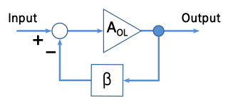
A negative-feedback amplifier is an electronic amplifier that subtracts a fraction of its output from its input, so that negative feedback opposes the original signal. The applied negative feedback can improve its performance and reduces sensitivity to parameter variations due to manufacturing or environment. Because of these advantages, many amplifiers and control systems use negative feedback.

Negative feedback occurs when some function of the output of a system, process, or mechanism is fed back in a manner that tends to reduce the fluctuations in the output, whether caused by changes in the input or by other disturbances. A classic example of negative feedback is a heating system thermostat — when the temperature gets high enough, the heater is turned OFF. When the temperature gets too cold, the heat is turned back ON. In each case the "feedback" generated by the thermostat "negates" the trend.

In control theory and stability theory, root locus analysis is a graphical method for examining how the roots of a system change with variation of a certain system parameter, commonly a gain within a feedback system. This is a technique used as a stability criterion in the field of classical control theory developed by Walter R. Evans which can determine stability of the system. The root locus plots the poles of the closed loop transfer function in the complex s-plane as a function of a gain parameter.

The step response of a system in a given initial state consists of the time evolution of its outputs when its control inputs are Heaviside step functions. In electronic engineering and control theory, step response is the time behaviour of the outputs of a general system when its inputs change from zero to one in a very short time. The concept can be extended to the abstract mathematical notion of a dynamical system using an evolution parameter.
Digital control is a branch of control theory that uses digital computers to act as system controllers. Depending on the requirements, a digital control system can take the form of a microcontroller to an ASIC to a standard desktop computer. Since a digital computer is a discrete system, the Laplace transform is replaced with the Z-transform. Since a digital computer has finite precision, extra care is needed to ensure the error in coefficients, analog-to-digital conversion, digital-to-analog conversion, etc. are not producing undesired or unplanned effects.

A closed-loop controller or feedback controller is a control loop which incorporates feedback, in contrast to an open-loop controller or non-feedback controller. A closed-loop controller uses feedback to control states or outputs of a dynamical system. Its name comes from the information path in the system: process inputs have an effect on the process outputs, which is measured with sensors and processed by the controller; the result is "fed back" as input to the process, closing the loop.
Infinite impulse response (IIR) is a property applying to many linear time-invariant systems that are distinguished by having an impulse response that does not become exactly zero past a certain point but continues indefinitely. This is in contrast to a finite impulse response (FIR) system, in which the impulse response does become exactly zero at times for some finite , thus being of finite duration. Common examples of linear time-invariant systems are most electronic and digital filters. Systems with this property are known as IIR systems or IIR filters.
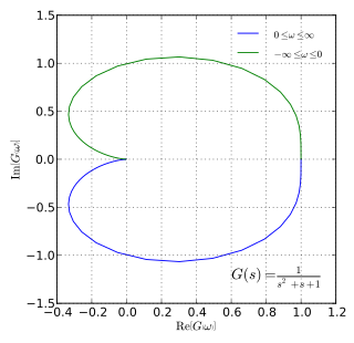
In control theory and stability theory, the Nyquist stability criterion or Strecker–Nyquist stability criterion, independently discovered by the German electrical engineer Felix Strecker at Siemens in 1930 and the Swedish-American electrical engineer Harry Nyquist at Bell Telephone Laboratories in 1932, is a graphical technique for determining the stability of a dynamical system.
In control theory, quantitative feedback theory (QFT), developed by Isaac Horowitz, is a frequency domain technique utilising the Nichols chart (NC) in order to achieve a desired robust design over a specified region of plant uncertainty. Desired time-domain responses are translated into frequency domain tolerances, which lead to bounds on the loop transmission function. The design process is highly transparent, allowing a designer to see what trade-offs are necessary to achieve a desired performance level.
A lead–lag compensator is a component in a control system that improves an undesirable frequency response in a feedback and control system. It is a fundamental building block in classical control theory.
In discrete-time control theory, the dead-beat control problem consists of finding what input signal must be applied to a system in order to bring the output to the steady state in the smallest number of time steps.
In systems theory, closed-loop poles are the positions of the poles of a closed-loop transfer function in the s-plane. The open-loop transfer function is equal to the product of all transfer function blocks in the forward path in the block diagram. The closed-loop transfer function is obtained by dividing the open-loop transfer function by the sum of one and the product of all transfer function blocks throughout the negative feedback loop. The closed-loop transfer function may also be obtained by algebraic or block diagram manipulation. Once the closed-loop transfer function is obtained for the system, the closed-loop poles are obtained by solving the characteristic equation. The characteristic equation is nothing more than setting the denominator of the closed-loop transfer function to zero.
A signal-flow graph or signal-flowgraph (SFG), invented by Claude Shannon, but often called a Mason graph after Samuel Jefferson Mason who coined the term, is a specialized flow graph, a directed graph in which nodes represent system variables, and branches represent functional connections between pairs of nodes. Thus, signal-flow graph theory builds on that of directed graphs, which includes as well that of oriented graphs. This mathematical theory of digraphs exists, of course, quite apart from its applications.
Classical control theory is a branch of control theory that deals with the behavior of dynamical systems with inputs, and how their behavior is modified by feedback, using the Laplace transform as a basic tool to model such systems.


