Condensation algorithm

Last updated June 15, 2024

The condensation algorithm (Conditional Density Propagation) is a computer vision algorithm. The principal application is to detect and track the contour of objects moving in a cluttered environment. Object tracking is one of the more basic and difficult aspects of computer vision and is generally a prerequisite to object recognition. Being able to identify which pixels in an image make up the contour of an object is a non-trivial problem. Condensation is a probabilistic algorithm that attempts to solve this problem.

The algorithm itself is described in detail by Isard and Blake in a publication in the International Journal of Computer Vision in 1998.^[1] One of the most interesting facets of the algorithm is that it does not compute on every pixel of the image. Rather, pixels to process are chosen at random, and only a subset of the pixels end up being processed. Multiple hypotheses about what is moving are supported naturally by the probabilistic nature of the approach. The evaluation functions come largely from previous work in the area and include many standard statistical approaches. The original part of this work is the application of particle filter estimation techniques.

The algorithm’s creation was inspired by the inability of Kalman filtering to perform object tracking well in the presence of significant background clutter. The presence of clutter tends to produce probability distributions for the object state which are multi-modal and therefore poorly modeled by the Kalman filter. The condensation algorithm in its most general form requires no assumptions about the probability distributions of the object or measurements.

Algorithm overview

The condensation algorithm seeks to solve the problem of estimating the conformation of an object described by a vector $\mathbf {x_{t}}$ at time $t$ , given observations $\mathbf {z_{1},...,z_{t}}$ of the detected features in the images up to and including the current time. The algorithm outputs an estimate to the state conditional probability density $p(\mathbf {x_{t}} |\mathbf {z_{1},...,z_{t}} )$ by applying a nonlinear filter based on factored sampling and can be thought of as a development of a Monte-Carlo method.^[1] $p(\mathbf {x_{t}} |\mathbf {z_{1},...,z_{t}} )$ is a representation of the probability of possible conformations for the objects based on previous conformations and measurements. The condensation algorithm is a generative model ^[2] since it models the joint distribution of the object and the observer.

The conditional density of the object at the current time $p(\mathbf {x_{t}} |\mathbf {z_{1},...,z_{t}} )$ is estimated as a weighted, time-indexed sample set $\{s_{t}^{(n)},n=1,...,N\}$ with weights $\pi _{t}^{(n)}$ . N is a parameter determining the number of sample sets chosen. A realization of $p(\mathbf {x_{t}} |\mathbf {z_{1},...,z_{t}} )$ is obtained by sampling with replacement from the set $s_{t}$ with probability equal to the corresponding element of $\pi _{t}$ .^[1]

The assumptions that object dynamics form a temporal Markov chain and that observations are independent of each other and the dynamics facilitate the implementation of the condensation algorithm. The first assumption allows the dynamics of the object to be entirely determined by the conditional density $p(\mathbf {x_{t}} |\mathbf {x_{t-1}} )$ . The model of the system dynamics determined by $p(\mathbf {x_{t}} |\mathbf {x_{t-1}} )$ must also be selected for the algorithm, and generally includes both deterministic and stochastic dynamics.

The algorithm can be summarized by initialization at time $t=0$ and three steps at each time t:

Initialization

Form the initial sample set and weights by sampling according to the prior distribution. For example, specify as Gaussian and set the weights equal to each other.

Iterative procedure

Sample with replacement $N$ times from the set $\{s_{0}^{(n)},n=1,...,N\}$ with probability $\{\pi _{0}^{(n)},n=1,...,N\}$ to generate a realization of $p(\mathbf {x_{t}} |\mathbf {z_{1},...,z_{t}} )$ .
Apply the learned dynamics $p(\mathbf {x_{t}} |\mathbf {x_{t-1}} )$ to each element of this new set, to generate a new set $\{s_{t}^{(n)}\}$ .
To take into account the current observation $\mathbf {z_{t}}$ , set $\pi _{t}^{(n)}={\frac {p(\mathbf {z_{t}} |s^{(n)})}{\sum _{j=1}^{N}p(\mathbf {z_{t}} |s^{(j)})}}$ for each element $\{s_{t}^{(n)}\}$ .

This algorithm outputs the probability distribution $p(\mathbf {x_{t}} |\mathbf {z_{1},...,z_{t}} )$ which can be directly used to calculate the mean position of the tracked object, as well as the other moments of the tracked object.

Cumulative weights can instead be used to achieve a more efficient sampling.^[1]

Implementation considerations

Since object-tracking can be a real-time objective, consideration of algorithm efficiency becomes important. The condensation algorithm is relatively simple when compared to the computational intensity of the Ricatti equation required for Kalman filtering. The parameter $N$ , which determines the number of samples in the sample set, will clearly hold a trade-off in efficiency versus performance.

One way to increase efficiency of the algorithm is by selecting a low degree of freedom model for representing the shape of the object. The model used by Isard 1998 is a linear parameterization of B-splines in which the splines are limited to certain configurations. Suitable configurations were found by analytically determining combinations of contours from multiple views, of the object in different poses, and through principal component analysis (PCA) on the deforming object.

Isard and Blake model the object dynamics $p(\mathbf {x_{t}} |\mathbf {x_{t-1}} )$ as a second order difference equation with deterministic and stochastic components: $p(\mathbf {x_{t}} |\mathbf {x_{t-1}} )\propto e^{-{\frac {1}{2}}||B^{-1}((\mathbf {x_{t}} -\mathbf {\bar {x}} )-A(\mathbf {x_{t-1}} -\mathbf {\bar {x}} ))||^{2})}$

where $\mathbf {\bar {x}}$ is the mean value of the state, and $A$ , $B$ are matrices representing the deterministic and stochastic components of the dynamical model respectively. $A$ , $B$ , and $\mathbf {\bar {x}}$ are estimated via Maximum Likelihood Estimation while the object performs typical movements.^[1]^[3]

The observation model $p(\mathbf {z} |\mathbf {x} )$ cannot be directly estimated from the data, requiring assumptions to be made in order to estimate it. Isard 1998 assumes that the clutter which may make the object not visible is a Poisson random process with spatial density $\lambda$ and that any true target measurement is unbiased and normally distributed with standard deviation $\sigma$ .

The basic condensation algorithm is used to track a single object in time. It is possible to extend the condensation algorithm using a single probability distribution to describe the likely states of multiple objects to track multiple objects in a scene at the same time.^[4]

Since clutter can cause the object probability distribution to split into multiple peaks, each peak represents a hypothesis about the object configuration. Smoothing is a statistical technique of conditioning the distribution based on both past and future measurements once the tracking is complete in order to reduce the effects of multiple peaks.^[5] Smoothing cannot be directly done in real-time since it requires information of future measurements.

Applications

The algorithm can be used for vision-based robot localization of mobile robots.^[6] Instead of tracking the position of an object in the scene, however, the position of the camera platform is tracked. This allows the camera platform to be globally localized given a visual map of the environment.

Extensions of the condensation algorithm have also been used to recognize human gestures in image sequences. This application of the condensation algorithm impacts the range of human–computer interactions possible. It has been used to recognize simple gestures of a user at a whiteboard to control actions such as selecting regions of the boards to print or save them.^[7] Other extensions have also been used for tracking multiple cars in the same scene.^[8]

The condensation algorithm has also been used for face recognition in a video sequence.^[9]

Resources

An implementation of the condensation algorithm in C can be found on Michael Isard’s website.

An implementation in MATLAB can be found on the Mathworks File Exchange.

An example of implementation using the OpenCV library can be found on the OpenCV forums.

Related Research Articles

In probability theory and statistics, a normal distribution or Gaussian distribution is a type of continuous probability distribution for a real-valued random variable. The general form of its probability density function is

In probability theory, a probability density function (PDF), density function, or density of an absolutely continuous random variable, is a function whose value at any given sample in the sample space can be interpreted as providing a relative likelihood that the value of the random variable would be equal to that sample. Probability density is the probability per unit length, in other words, while the absolute likelihood for a continuous random variable to take on any particular value is 0, the value of the PDF at two different samples can be used to infer, in any particular draw of the random variable, how much more likely it is that the random variable would be close to one sample compared to the other sample.

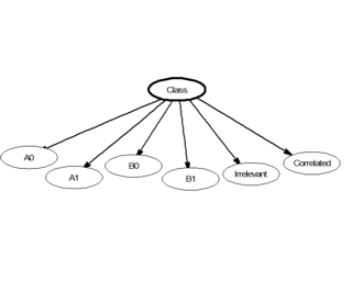
In statistics, naive Bayes classifiers are a family of linear "probabilistic classifiers" which assumes that the features are conditionally independent, given the target class. The strength (naivety) of this assumption is what gives the classifier its name. These classifiers are among the simplest Bayesian network models.

For statistics and control theory, Kalman filtering, also known as linear quadratic estimation (LQE), is an algorithm that uses a series of measurements observed over time, including statistical noise and other inaccuracies, and produces estimates of unknown variables that tend to be more accurate than those based on a single measurement alone, by estimating a joint probability distribution over the variables for each timeframe. The filter is named after Rudolf E. Kálmán, who was one of the primary developers of its theory.

In statistics, an expectation–maximization (EM) algorithm is an iterative method to find (local) maximum likelihood or maximum a posteriori (MAP) estimates of parameters in statistical models, where the model depends on unobserved latent variables. The EM iteration alternates between performing an expectation (E) step, which creates a function for the expectation of the log-likelihood evaluated using the current estimate for the parameters, and a maximization (M) step, which computes parameters maximizing the expected log-likelihood found on the E step. These parameter-estimates are then used to determine the distribution of the latent variables in the next E step. It can be used, for example, to estimate a mixture of gaussians, or to solve the multiple linear regression problem.

In statistics, Gibbs sampling or a Gibbs sampler is a Markov chain Monte Carlo (MCMC) algorithm for sampling from a specified multivariate probability distribution when direct sampling from the joint distribution is difficult, but sampling from the conditional distribution is more practical. This sequence can be used to approximate the joint distribution ; to approximate the marginal distribution of one of the variables, or some subset of the variables ; or to compute an integral. Typically, some of the variables correspond to observations whose values are known, and hence do not need to be sampled.

In signal processing, independent component analysis (ICA) is a computational method for separating a multivariate signal into additive subcomponents. This is done by assuming that at most one subcomponent is Gaussian and that the subcomponents are statistically independent from each other. ICA was invented by Jeanny Hérault and Christian Jutten in 1985. ICA is a special case of blind source separation. A common example application of ICA is the "cocktail party problem" of listening in on one person's speech in a noisy room.

Statistical learning theory is a framework for machine learning drawing from the fields of statistics and functional analysis. Statistical learning theory deals with the statistical inference problem of finding a predictive function based on data. Statistical learning theory has led to successful applications in fields such as computer vision, speech recognition, and bioinformatics.

Video tracking is the process of locating a moving object over time using a camera. It has a variety of uses, some of which are: human-computer interaction, security and surveillance, video communication and compression, augmented reality, traffic control, medical imaging and video editing. Video tracking can be a time-consuming process due to the amount of data that is contained in video. Adding further to the complexity is the possible need to use object recognition techniques for tracking, a challenging problem in its own right.

Probability theory and statistics have some commonly used conventions, in addition to standard mathematical notation and mathematical symbols.

Conditional random fields (CRFs) are a class of statistical modeling methods often applied in pattern recognition and machine learning and used for structured prediction. Whereas a classifier predicts a label for a single sample without considering "neighbouring" samples, a CRF can take context into account. To do so, the predictions are modelled as a graphical model, which represents the presence of dependencies between the predictions. What kind of graph is used depends on the application. For example, in natural language processing, "linear chain" CRFs are popular, for which each prediction is dependent only on its immediate neighbours. In image processing, the graph typically connects locations to nearby and/or similar locations to enforce that they receive similar predictions.

The cross-entropy (CE) method is a Monte Carlo method for importance sampling and optimization. It is applicable to both combinatorial and continuous problems, with either a static or noisy objective.

Mean shift is a non-parametric feature-space mathematical analysis technique for locating the maxima of a density function, a so-called mode-seeking algorithm. Application domains include cluster analysis in computer vision and image processing.

<span class="mw-page-title-main">Active contour model</span>

Active contour model, also called snakes, is a framework in computer vision introduced by Michael Kass, Andrew Witkin, and Demetri Terzopoulos for delineating an object outline from a possibly noisy 2D image. The snakes model is popular in computer vision, and snakes are widely used in applications like object tracking, shape recognition, segmentation, edge detection and stereo matching.

In statistics, the Bingham distribution, named after Christopher Bingham, is an antipodally symmetric probability distribution on the n-sphere. It is a generalization of the Watson distribution and a special case of the Kent and Fisher–Bingham distributions.

In cryptography, learning with errors (LWE) is a mathematical problem that is widely used to create secure encryption algorithms. It is based on the idea of representing secret information as a set of equations with errors. In other words, LWE is a way to hide the value of a secret by introducing noise to it. In more technical terms, it refers to the computational problem of inferring a linear $-ary function over a finite ring from given samples some of which may be erroneous. The LWE problem is conjectured to be hard to solve, and thus to be useful in cryptography.$

t-distributed stochastic neighbor embedding (t-SNE) is a statistical method for visualizing high-dimensional data by giving each datapoint a location in a two or three-dimensional map. It is based on Stochastic Neighbor Embedding originally developed by Geoffrey Hinton and Sam Roweis, where Laurens van der Maaten proposed the t-distributed variant. It is a nonlinear dimensionality reduction technique for embedding high-dimensional data for visualization in a low-dimensional space of two or three dimensions. Specifically, it models each high-dimensional object by a two- or three-dimensional point in such a way that similar objects are modeled by nearby points and dissimilar objects are modeled by distant points with high probability.

In machine learning, the kernel embedding of distributions comprises a class of nonparametric methods in which a probability distribution is represented as an element of a reproducing kernel Hilbert space (RKHS). A generalization of the individual data-point feature mapping done in classical kernel methods, the embedding of distributions into infinite-dimensional feature spaces can preserve all of the statistical features of arbitrary distributions, while allowing one to compare and manipulate distributions using Hilbert space operations such as inner products, distances, projections, linear transformations, and spectral analysis. This learning framework is very general and can be applied to distributions over any space $on which a sensible kernel function may be defined. For example, various kernels have been proposed for learning from data which are: vectors in, discrete classes/categories, strings, graphs/networks, images, time series, manifolds, dynamical systems, and other structured objects. The theory behind kernel embeddings of distributions has been primarily developed by Alex Smola, Le Song, Arthur Gretton, and Bernhard Schölkopf. A review of recent works on kernel embedding of distributions can be found in.$

Mean-field particle methods are a broad class of interacting type Monte Carlo algorithms for simulating from a sequence of probability distributions satisfying a nonlinear evolution equation. These flows of probability measures can always be interpreted as the distributions of the random states of a Markov process whose transition probabilities depends on the distributions of the current random states. A natural way to simulate these sophisticated nonlinear Markov processes is to sample a large number of copies of the process, replacing in the evolution equation the unknown distributions of the random states by the sampled empirical measures. In contrast with traditional Monte Carlo and Markov chain Monte Carlo methods these mean-field particle techniques rely on sequential interacting samples. The terminology mean-field reflects the fact that each of the samples interacts with the empirical measures of the process. When the size of the system tends to infinity, these random empirical measures converge to the deterministic distribution of the random states of the nonlinear Markov chain, so that the statistical interaction between particles vanishes. In other words, starting with a chaotic configuration based on independent copies of initial state of the nonlinear Markov chain model, the chaos propagates at any time horizon as the size the system tends to infinity; that is, finite blocks of particles reduces to independent copies of the nonlinear Markov process. This result is called the propagation of chaos property. The terminology "propagation of chaos" originated with the work of Mark Kac in 1976 on a colliding mean-field kinetic gas model.

Dependency networks (DNs) are graphical models, similar to Markov networks, wherein each vertex (node) corresponds to a random variable and each edge captures dependencies among variables. Unlike Bayesian networks, DNs may contain cycles. Each node is associated to a conditional probability table, which determines the realization of the random variable given its parents.

References

1 2 3 4 5 Isard, M.; Blake, A (August 1998). "CONDENSATION-- conditional density propagation of visual tracking". International Journal of Computer Vision. 29 (1): 5–28. doi:10.1023/A:1008078328650. S2CID 6821810.
↑ Sminchisescu, C.; Kanaujia, A.; Metaxas, D.N. (November 2007). "BM3E: Discriminative Density Propagation for Visual Tracking". IEEE Transactions on Pattern Analysis and Machine Intelligence. 29 (11): 2030–2044. CiteSeerX 10.1.1.78.1751 . doi:10.1109/tpami.2007.1111. PMID 17848782. S2CID 1949783.
↑ Blake, Andrea; Isard, Michael; Reynard, David (October 1995). "Learning to track the visual motion of contours". Artificial Intelligence. 78 (1–2): 179–212. doi: 10.1016/0004-3702(95)00032-1 .
↑ Koller-Meier, Esther B.; Ade, Frank (28 February 2001). "Tracking multiple objects using the Condensation algorithm". Robotics and Autonomous Systems. 34 (2–3): 93–105. doi:10.1016/s0921-8890(00)00114-7.
↑ Isard, Michael; Blake, Andrew (28 May 2006). "A smoothing filter for condensation". Computer Vision — ECCV'98. Lecture Notes in Computer Science. Vol. 1406. pp. 767–781. doi:10.1007/BFb0055703. ISBN 978-3-540-64569-6.
↑ Dellaert, F.; Burgard, W.; Fox, D.; Thrun, S. (1999). "Using the CONDENSATION algorithm for robust, vision-based mobile robot localization". Proceedings. 1999 IEEE Computer Society Conference on Computer Vision and Pattern Recognition (Cat. No PR00149). Vol. 2. pp. 588–594. doi:10.1109/CVPR.1999.784976. hdl:1853/21565. ISBN 0-7695-0149-4. S2CID 16130780.{{cite book}}: |journal= ignored (help)
↑ Black, M.J.; Jepson, A.D. (14 April 1998). "Recognizing temporal trajectories using the condensation algorithm". Proceedings Third IEEE International Conference on Automatic Face and Gesture Recognition. pp. 16–21. CiteSeerX 10.1.1.154.1402 . doi:10.1109/AFGR.1998.670919. ISBN 0-8186-8344-9. S2CID 5159845.{{cite book}}: |journal= ignored (help)
↑ Meier, E.B.; Ade, Frank (1999). "Tracking cars in range images using the CONDENSATION algorithm". Proceedings 199 IEEE/IEEJ/JSAI International Conference on Intelligent Transportation Systems (Cat. No.99TH8383). pp. 129–134. doi:10.1109/ITSC.1999.821040. ISBN 0-7803-4975-X. S2CID 12548469.{{cite book}}: |journal= ignored (help)
↑ Zhou, Shaohua; Krueger, V.; Chellappa, R. (21 May 2002). "Face recognition from video: A CONDENSATION approach". Proceedings of Fifth IEEE International Conference on Automatic Face Gesture Recognition. pp. 221–226. doi:10.1109/AFGR.2002.1004158. ISBN 0-7695-1602-5. S2CID 8505547.{{cite book}}: |journal= ignored (help)

This page is based on this Wikipedia article
Text is available under the CC BY-SA 4.0 license; additional terms may apply.
Images, videos and audio are available under their respective licenses.

[Isard1998-1] 1 2 3 4 5 Isard, M.; Blake, A (August 1998). "CONDENSATION-- conditional density propagation of visual tracking". International Journal of Computer Vision. 29 (1): 5–28. doi:10.1023/A:1008078328650. S2CID 6821810.

[2] Sminchisescu, C.; Kanaujia, A.; Metaxas, D.N. (November 2007). "BM3E: Discriminative Density Propagation for Visual Tracking". IEEE Transactions on Pattern Analysis and Machine Intelligence. 29 (11): 2030–2044. CiteSeerX 10.1.1.78.1751 . doi:10.1109/tpami.2007.1111. PMID 17848782. S2CID 1949783.

[3] Blake, Andrea; Isard, Michael; Reynard, David (October 1995). "Learning to track the visual motion of contours". Artificial Intelligence. 78 (1–2): 179–212. doi: 10.1016/0004-3702(95)00032-1 .

[4] Koller-Meier, Esther B.; Ade, Frank (28 February 2001). "Tracking multiple objects using the Condensation algorithm". Robotics and Autonomous Systems. 34 (2–3): 93–105. doi:10.1016/s0921-8890(00)00114-7.

[5] Isard, Michael; Blake, Andrew (28 May 2006). "A smoothing filter for condensation". Computer Vision — ECCV'98. Lecture Notes in Computer Science. Vol. 1406. pp. 767–781. doi:10.1007/BFb0055703. ISBN 978-3-540-64569-6.

[6] Dellaert, F.; Burgard, W.; Fox, D.; Thrun, S. (1999). "Using the CONDENSATION algorithm for robust, vision-based mobile robot localization". Proceedings. 1999 IEEE Computer Society Conference on Computer Vision and Pattern Recognition (Cat. No PR00149). Vol. 2. pp. 588–594. doi:10.1109/CVPR.1999.784976. hdl:1853/21565. ISBN 0-7695-0149-4. S2CID 16130780.{{cite book}}: |journal= ignored (help)

[7] Black, M.J.; Jepson, A.D. (14 April 1998). "Recognizing temporal trajectories using the condensation algorithm". Proceedings Third IEEE International Conference on Automatic Face and Gesture Recognition. pp. 16–21. CiteSeerX 10.1.1.154.1402 . doi:10.1109/AFGR.1998.670919. ISBN 0-8186-8344-9. S2CID 5159845.{{cite book}}: |journal= ignored (help)

[8] Meier, E.B.; Ade, Frank (1999). "Tracking cars in range images using the CONDENSATION algorithm". Proceedings 199 IEEE/IEEJ/JSAI International Conference on Intelligent Transportation Systems (Cat. No.99TH8383). pp. 129–134. doi:10.1109/ITSC.1999.821040. ISBN 0-7803-4975-X. S2CID 12548469.{{cite book}}: |journal= ignored (help)

[9] Zhou, Shaohua; Krueger, V.; Chellappa, R. (21 May 2002). "Face recognition from video: A CONDENSATION approach". Proceedings of Fifth IEEE International Conference on Automatic Face Gesture Recognition. pp. 221–226. doi:10.1109/AFGR.2002.1004158. ISBN 0-7695-1602-5. S2CID 8505547.{{cite book}}: |journal= ignored (help)

[1]

[2]

[3]

[4]

[5]

[6]

[7]

[8]

[9]